Model and reconstruction settings
Reference solution
The plate spans 0–4 m in x and y and is clamped along its left edge. A uniform tension of 0.025 Pa acts on the right edge. The manuscript writes F = 0.025 N/m; its figures (far-field εxx ≈ 0.025, ux up to about 0.11 m) correspond to this edge stress. The reference is a plane-stress linear-triangle FE model with about 80,000 elements (element size 0.02 m); the manuscript used Q4 elements. The sensor data are this FE strain field sampled at the sensor positions, without noise.
Reconstruction
Each case runs the app's own steps 2–6. The PD points sit at the centres of a 0.04 m grid, each carrying the part of its cell inside the material. Strains are recovered with zeroth-order PD functions from the 16 nearest sensors (line of sight around the cutout). Displacements come from the least-squares construction with horizon 3Δx, weight δ²/|ξ|², μ = 1 at the sensor points and μ = 10⁻⁴ elsewhere, zero-energy-mode control α = 1, and the left edge clamped. The elastic constants follow from the reconstructed strains by the virtual fields method.
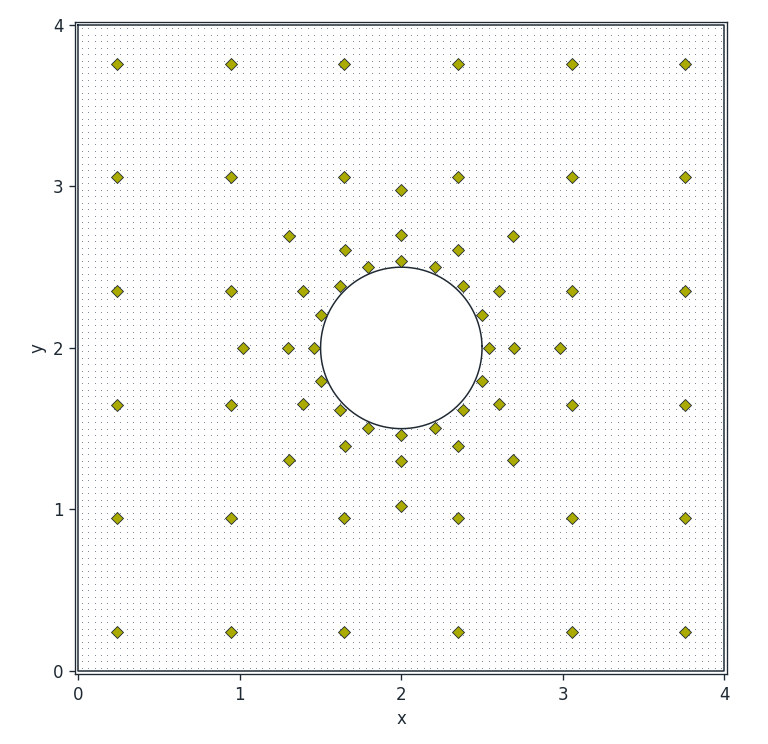
The sensors follow our own layout, which rings the cutout and adds a sparse grid in the far field.
Summary
Relative RMS error of each reconstructed field against the FE reference. For the circle the εxx error is 2.9 % and the ux error 0.8 %; the last column compares the largest ux with the FE value.
| Relative RMS error | |||||||
|---|---|---|---|---|---|---|---|
| Case | Sensors | εxx | εyy | γxy | ux | uy | Max ux [m] PDDO / FE |
| Circular cutout | 68/68 | 2.9 % | 4.8 % | 6.2 % | 0.8 % | 3.8 % | 0.1216 / 0.1245 |
| Inclined elliptical cutout | 82/82 | 3.6 % | 5.6 % | 5.6 % | 1.1 % | 2.1 % | 0.1188 / 0.1213 |
| Rectangular slit | 42/44 | 5.1 % | 7.8 % | 8.0 % | 4.5 % | 4.3 % | 0.1393 / 0.1326 |
3.1.1Circular cutout
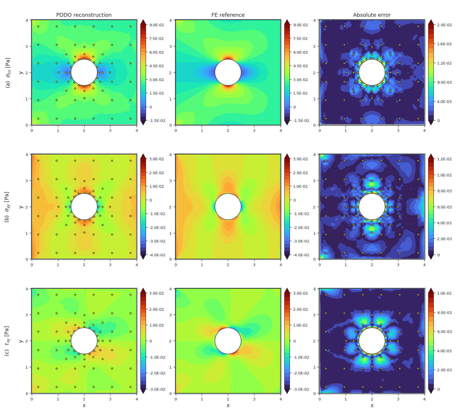
The cutout is a circle of radius r = 0.5 m, centred at (2, 2) m. The PD grid has 9,516 points (Δx = 0.04 m). The layout places 68 sensors.
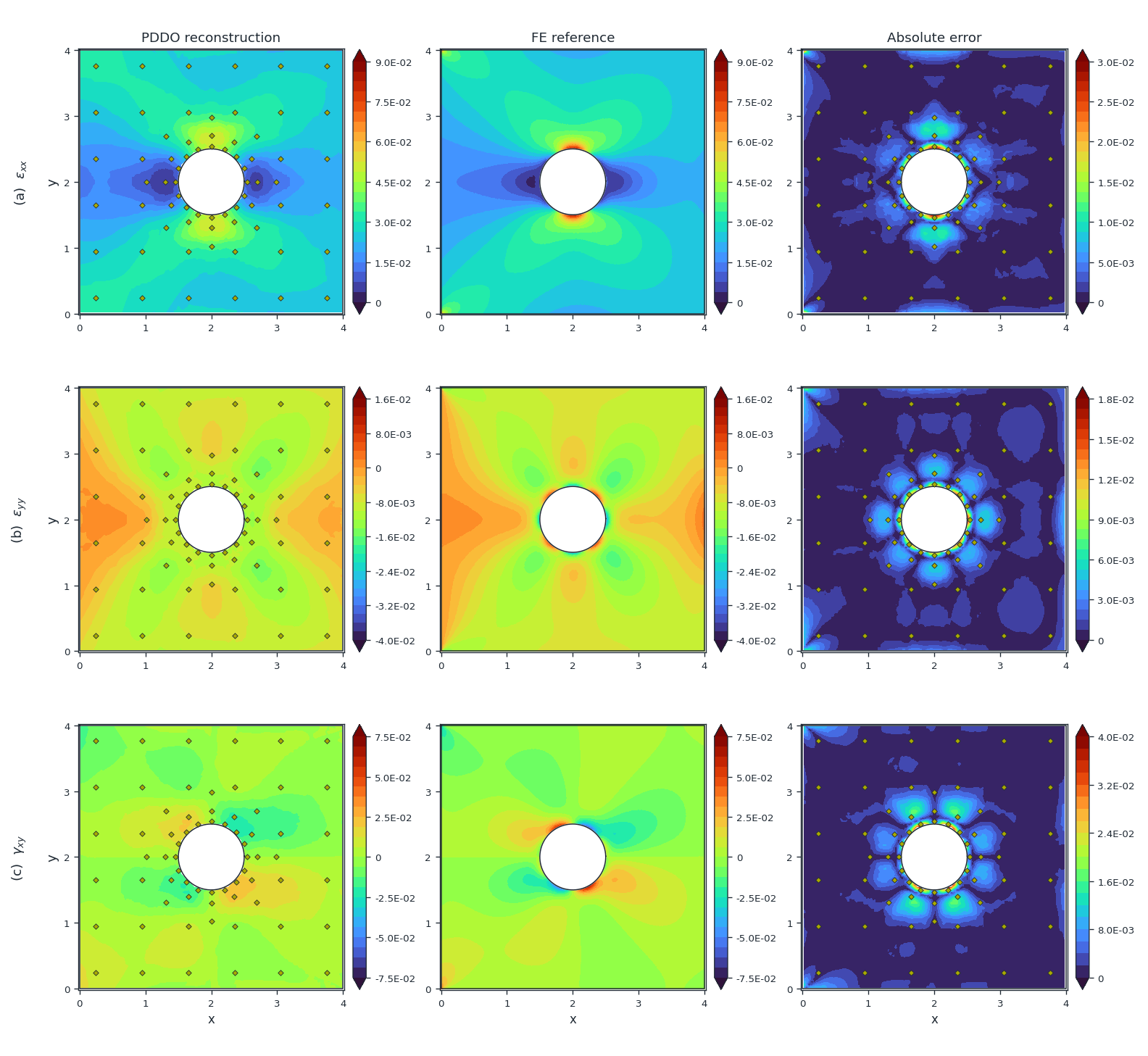
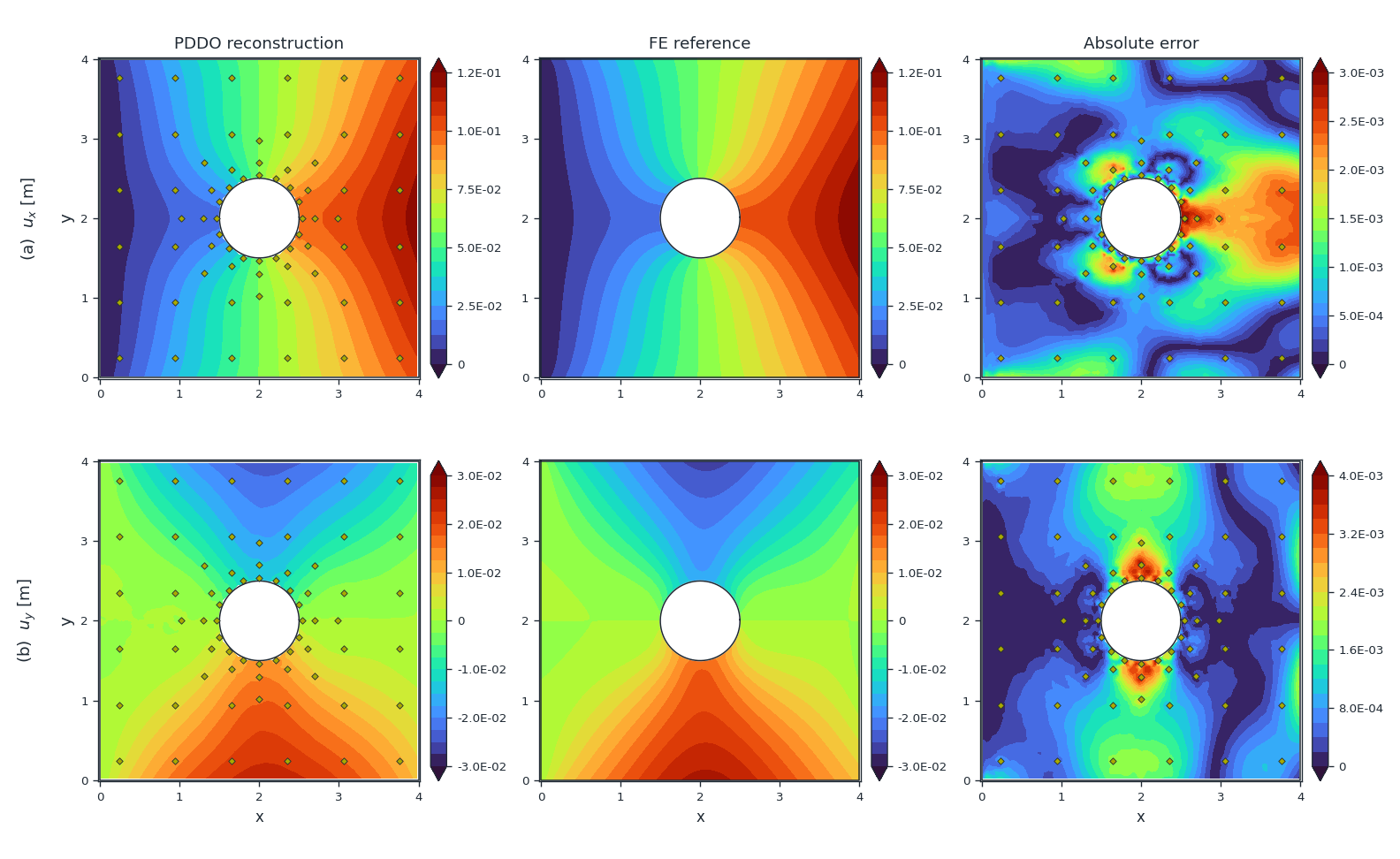
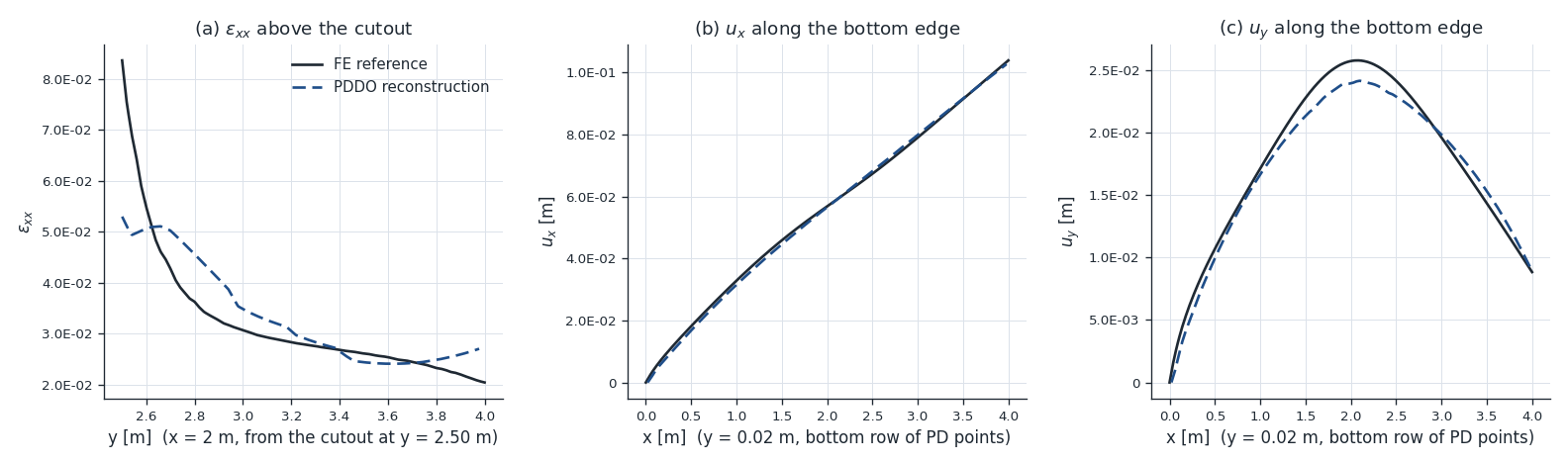
| Quantity | Rel. RMS | Max |error| |
|---|---|---|
| εxx | 2.9 % | 3.0e-02 |
| εyy | 4.8 % | 1.7e-02 |
| γxy | 6.2 % | 3.7e-02 |
| ux | 0.8 % | 2.9e-03 |
| uy | 3.8 % | 3.8e-03 |
Relative RMS: RMS of the error over the PD points, in % of the largest |FE value|. Strains are the recovered strains of step 4; displacements come from step 5.
3.1.2Inclined elliptical cutout
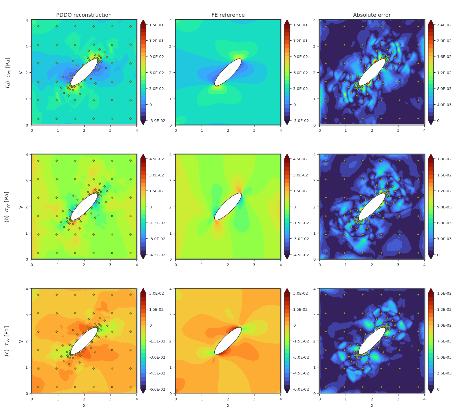
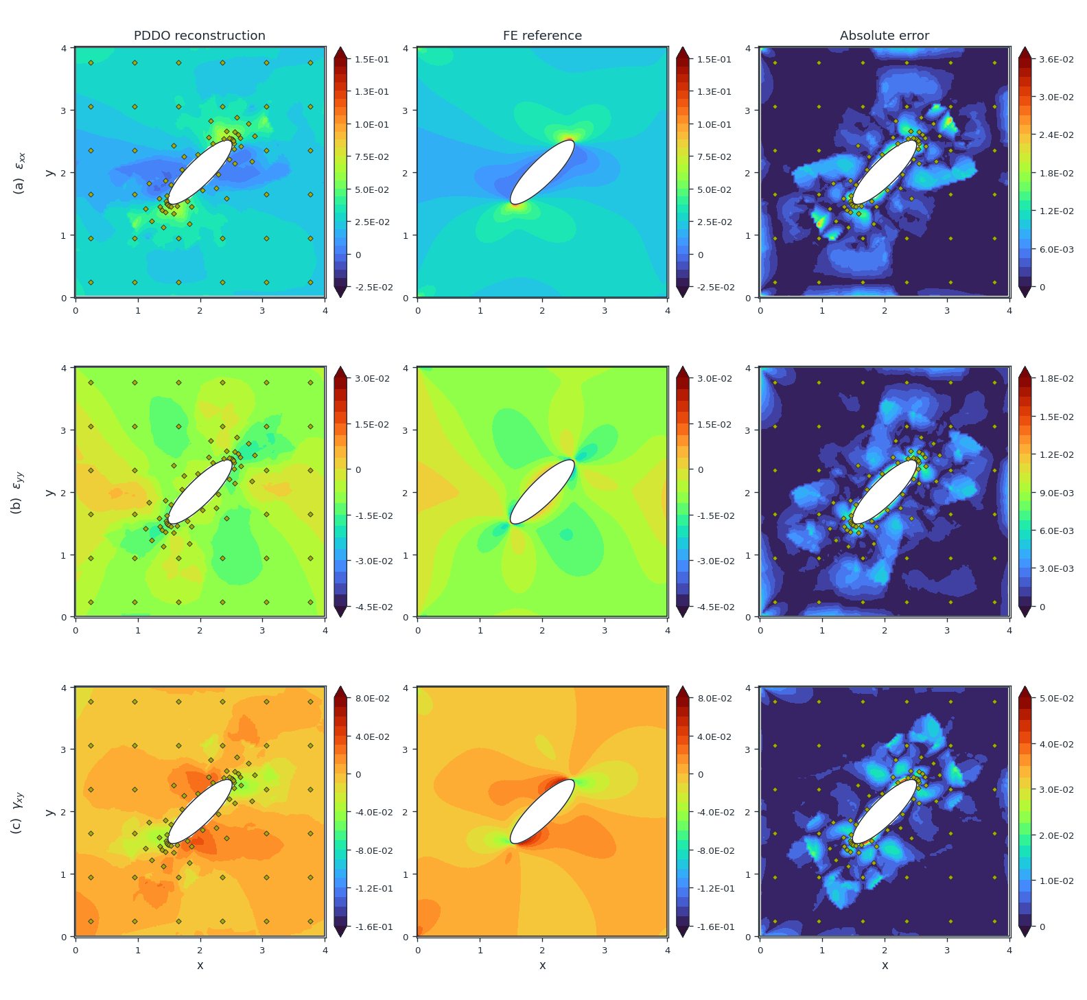
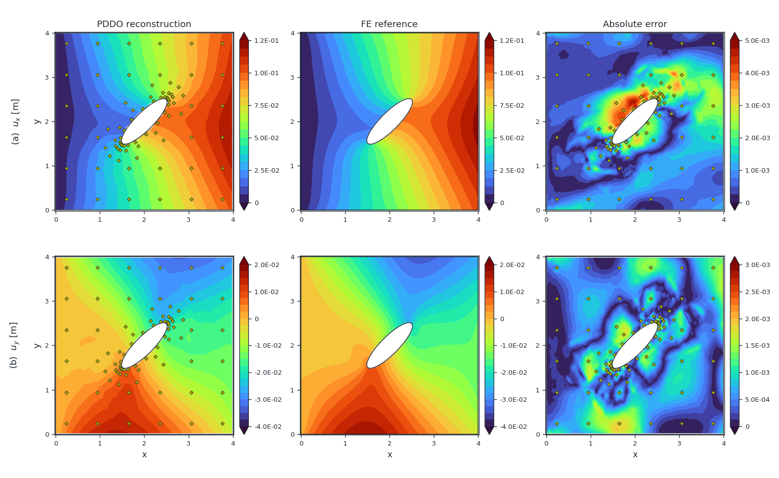
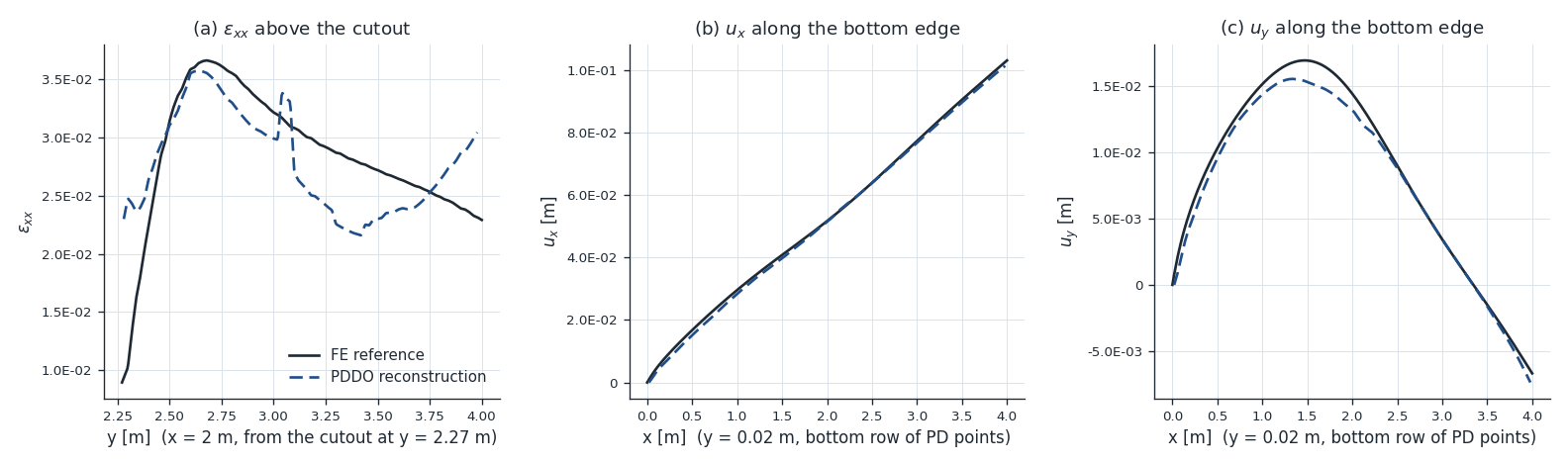
The cutout is an ellipse with semi-axes a = 0.7 m and b = 0.2 m, inclined 45° counter-clockwise from the x-axis, centred at (2, 2) m. The PD grid has 9,724 points (Δx = 0.04 m). The layout places 82 sensors.
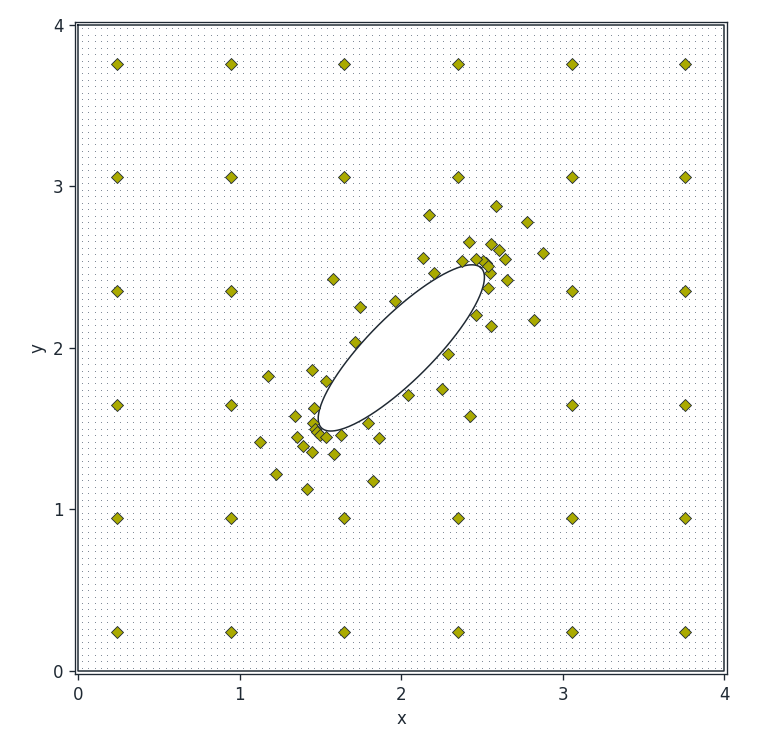
| Quantity | Rel. RMS | Max |error| |
|---|---|---|
| εxx | 3.6 % | 3.0e-02 |
| εyy | 5.6 % | 1.5e-02 |
| γxy | 5.6 % | 5.0e-02 |
| ux | 1.1 % | 4.9e-03 |
| uy | 2.1 % | 2.9e-03 |
Relative RMS: RMS of the error over the PD points, in % of the largest |FE value|. Strains are the recovered strains of step 4; displacements come from step 5.
3.1.3Rectangular slit
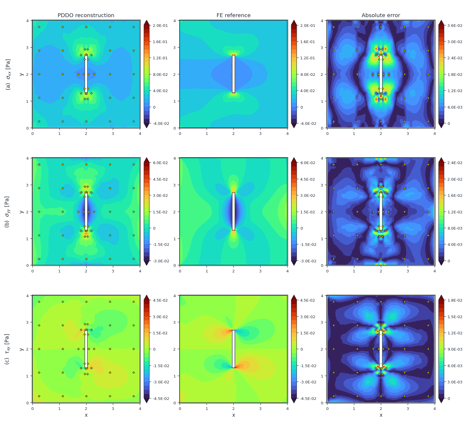
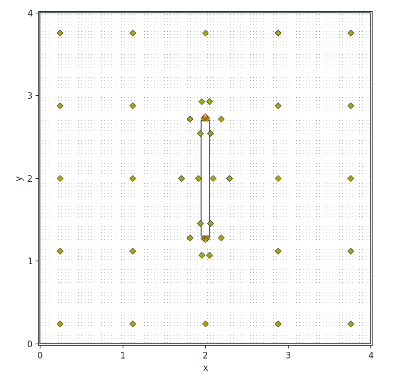
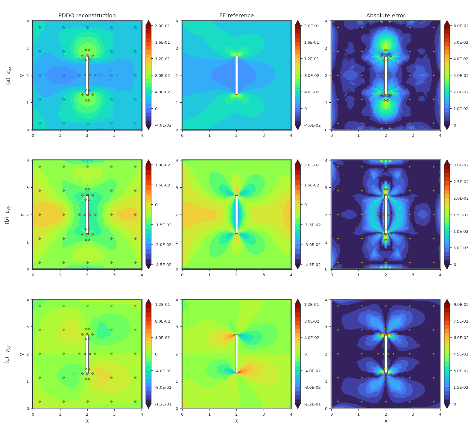
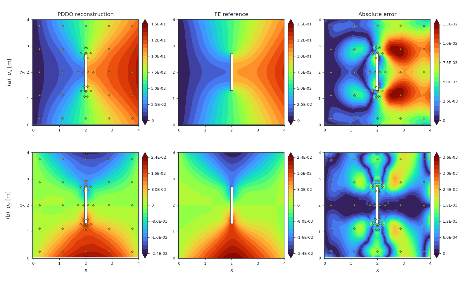
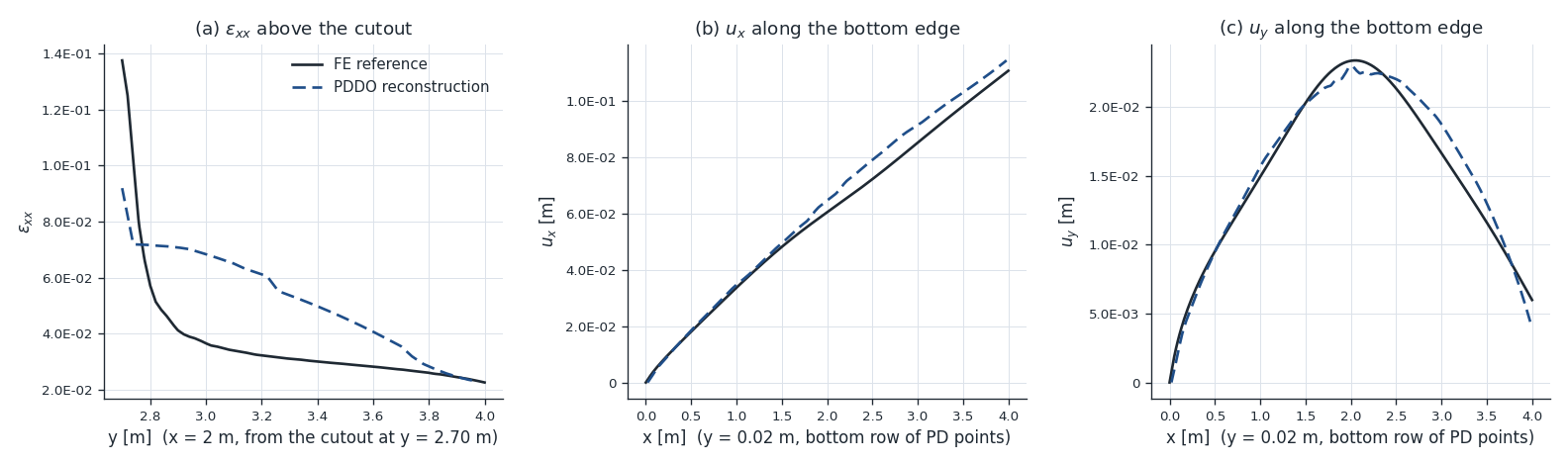
The cutout is a slit 1.4 m long and 0.1 m wide, aligned with the y-axis, centred at (2, 2) m. The PD grid has 9,930 points (Δx = 0.04 m). The layout places 42 of 44 sensors (2 share a PD point with a neighbouring sensor at Δx = 0.04 m and are skipped).
| Quantity | Rel. RMS | Max |error| |
|---|---|---|
| εxx | 5.1 % | 5.7e-02 |
| εyy | 7.8 % | 2.6e-02 |
| γxy | 8.0 % | 8.7e-02 |
| ux | 4.5 % | 1.2e-02 |
| uy | 4.3 % | 3.2e-03 |
Relative RMS: RMS of the error over the PD points, in % of the largest |FE value|. Strains are the recovered strains of step 4; displacements come from step 5.
3.1.4Material identification
The elastic constants are identified from the reconstructed strain field alone, with the principle of virtual work written over the PD points. For every admissible virtual field u*—zero on the supported edge, where the reaction is unknown, and rigid on the loaded edge, so that only the measured resultant does work—the internal and external virtual work must balance:
t Σk Ak σ(εk) · ε*k = F · u*(loaded edge)
Each field gives one linear equation in Q11 and Q12, and six polynomial fields are solved by least squares. Nothing but the strain field, the load resultant F = 0.01 N and the thickness t = 0.1 m enters; the FE solution is used only to check the answer. The virtual strains ε* = B u* are PDDO derivatives taken with the same operator that differentiates the reconstruction, which is exact for these quadratic fields.
The strains are those of the step-5 displacement field. Consistency is the largest disagreement between the six fields: they would all agree exactly on a field in equilibrium, so their spread measures how far the reconstruction is from one, without reference to the FE solution. The control column repeats the identification on the exact FE strains, which separates the error of the reconstruction from the error of the method.
| Identified from the reconstruction | Control | Stress error (rel. RMS) | |||||||
|---|---|---|---|---|---|---|---|---|---|
| Case | E [Pa] | Error | ν | Error | Consistency | E / ν, exact strains | σxx | σyy | τxy |
| Circular cutout | 0.999 | -0.1 % | 0.331 | -0.8 % | 0.61 % | 1.001 / 0.333 | 2.0 % | 3.8 % | 4.9 % |
| Inclined elliptical cutout | 1.018 | +1.8 % | 0.329 | -1.2 % | 0.55 % | 1.001 / 0.333 | 2.5 % | 5.7 % | 4.7 % |
| Rectangular slit | 0.918 | -8.2 % | 0.293 | -12.2 % | 0.47 % | 1.000 / 0.333 | 4.2 % | 7.9 % | 6.5 % |
The plate was generated with E = 1 Pa and ν = 0.3333 under plane stress. Stresses are the identified law applied to the reconstructed strains, against the FE strains through the true law.