Peridynamic Field Recovery
Full strain, displacement and stress fields — and the elastic constants — from a handful of strain gauges.
About
Peridynamic Field Recovery (PDRecovery) reconstructs the complete mechanical state of a structural component from strain measured at a small number of discrete points. Strain gauges, fibre-optic sensors and rosettes report a few dozen readings; PDRecovery turns them into continuous strain, displacement and stress fields over the whole part, including around the holes, notches and slits where the gradients matter most.
The engine is the Peridynamic Differential Operator (PDDO) — a non-local, mesh-free framework that integrates over a finite horizon instead of differencing neighbouring points. Because the domain is defined analytically and every sensor family is filtered by line of sight, no data is blended across a cut-out. The result needs no finite element model of the part, no material properties as input, and no expert interpolation of the gauge readings.
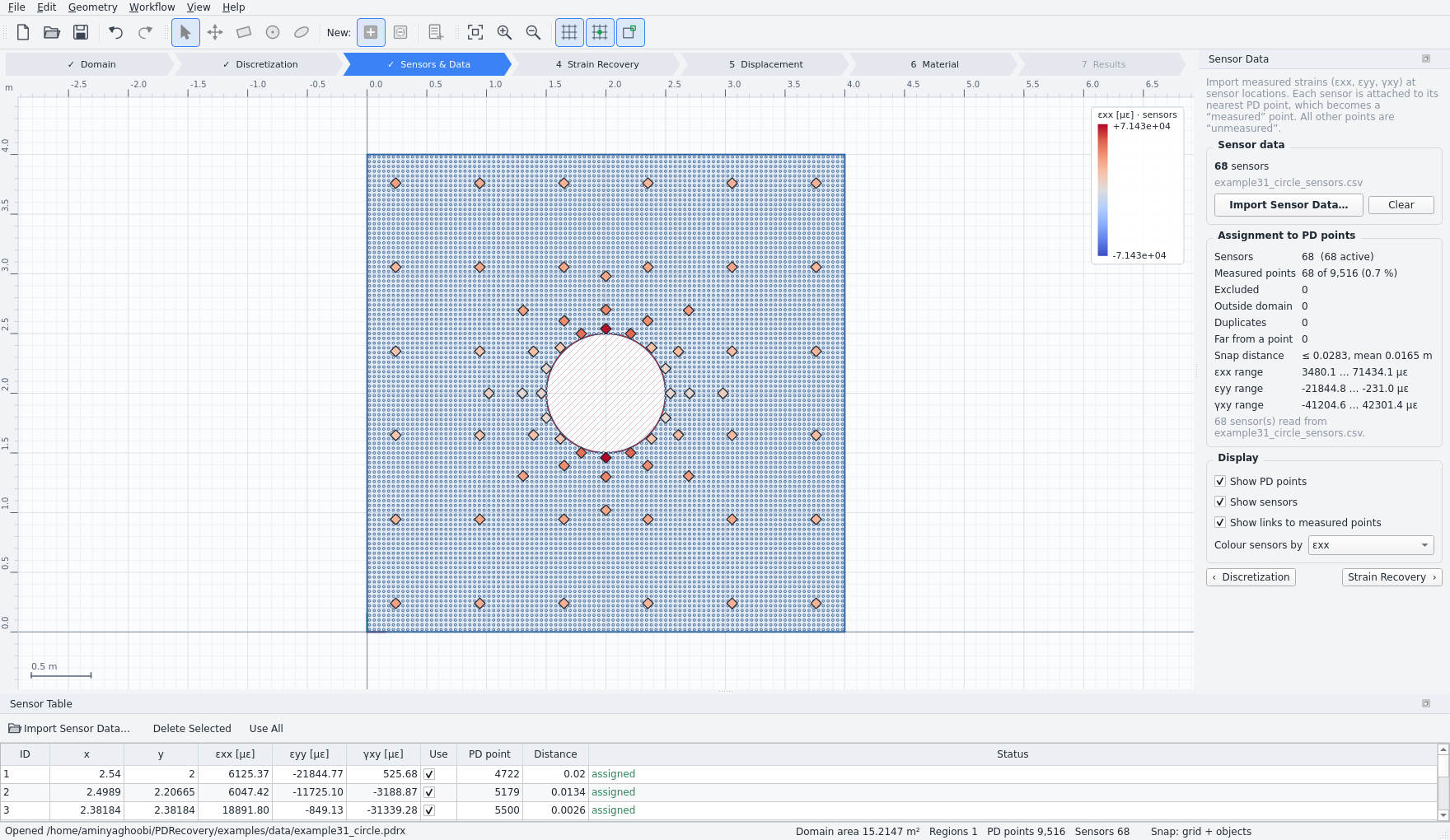 Steps 1–3. Domain, peridynamic discretization and the measured sensors, each attached to its nearest point.
How It Works
The part is discretized into peridynamic points carrying cell areas. Each sensor is attached to its nearest point and receives a lumped area from inverse-distance shares of the surrounding cells. The zeroth-order PDDO then estimates all three strain components at every point from the nearest sensors in line of sight, using a quadratic basis with Gaussian weights. Families whose sensors happen to lie on a single ring or curve are enlarged automatically until the estimator is well conditioned, so the reconstruction stays stable wherever the sensors happen to fall.
Displacements follow from a least-squares minimisation: the field whose peridynamic strains best match the measured values at the sensors and the recovered values everywhere else. Since nonlocal derivatives average over a family of neighbours, they barely see a displacement that alternates from point to point, and those near-zero-energy modes would otherwise be excited by measurement noise. A dedicated mode control penalises exactly what the peridynamic family cannot represent — and nothing it can — so the reconstruction comes out smooth without being smoothed.
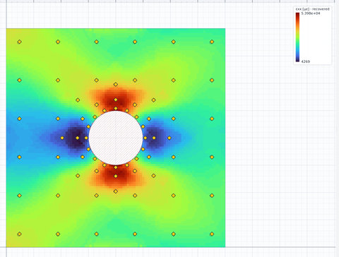
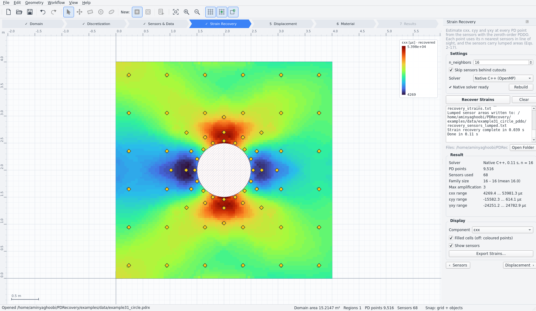 Step 4. Normal strain εxx recovered at 9,516 points from 68 sensors — the concentration at the hole resolves cleanly.
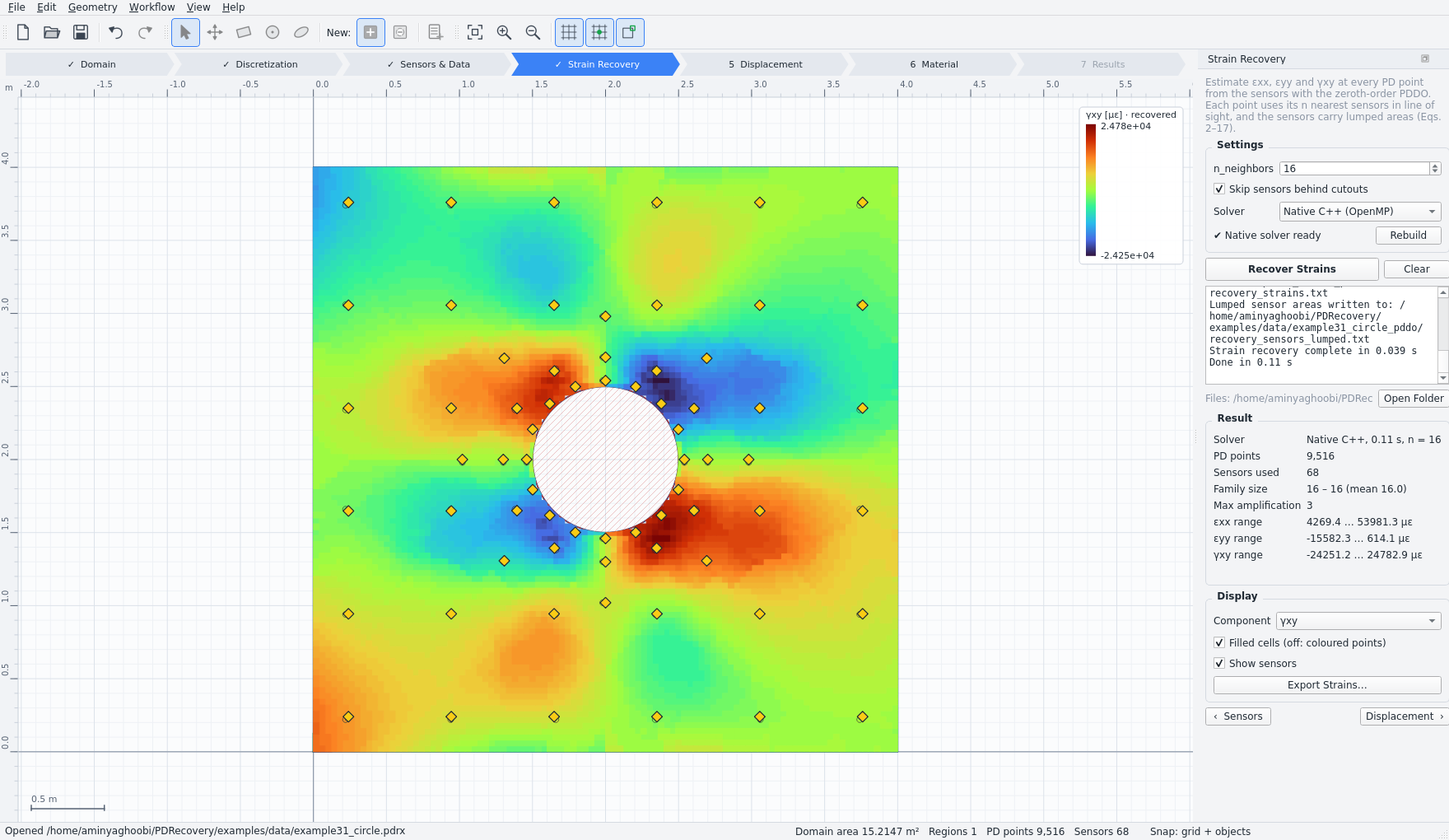 Step 4. Shear strain γxy over the same domain — the cut-out is never blended across.
Analysis Pipeline
- Domain: build the part from rectangles, circles and ellipses as parts and cut-outs
- Discretization: structured grid, body-fitted rings around holes, scattered points, or imported points
- Sensors and data: import measured strains from CSV or text, in strain, µε or %
- Strain recovery: zeroth-order PDDO with lumped sensor areas and line-of-sight families
- Displacement: peridynamic least-squares minimisation with zero-energy-mode control
- Material: E and ν by the virtual fields method from the reconstructed strains
- Results: stresses, von Mises, deformed shape, line profiles, and export of every field
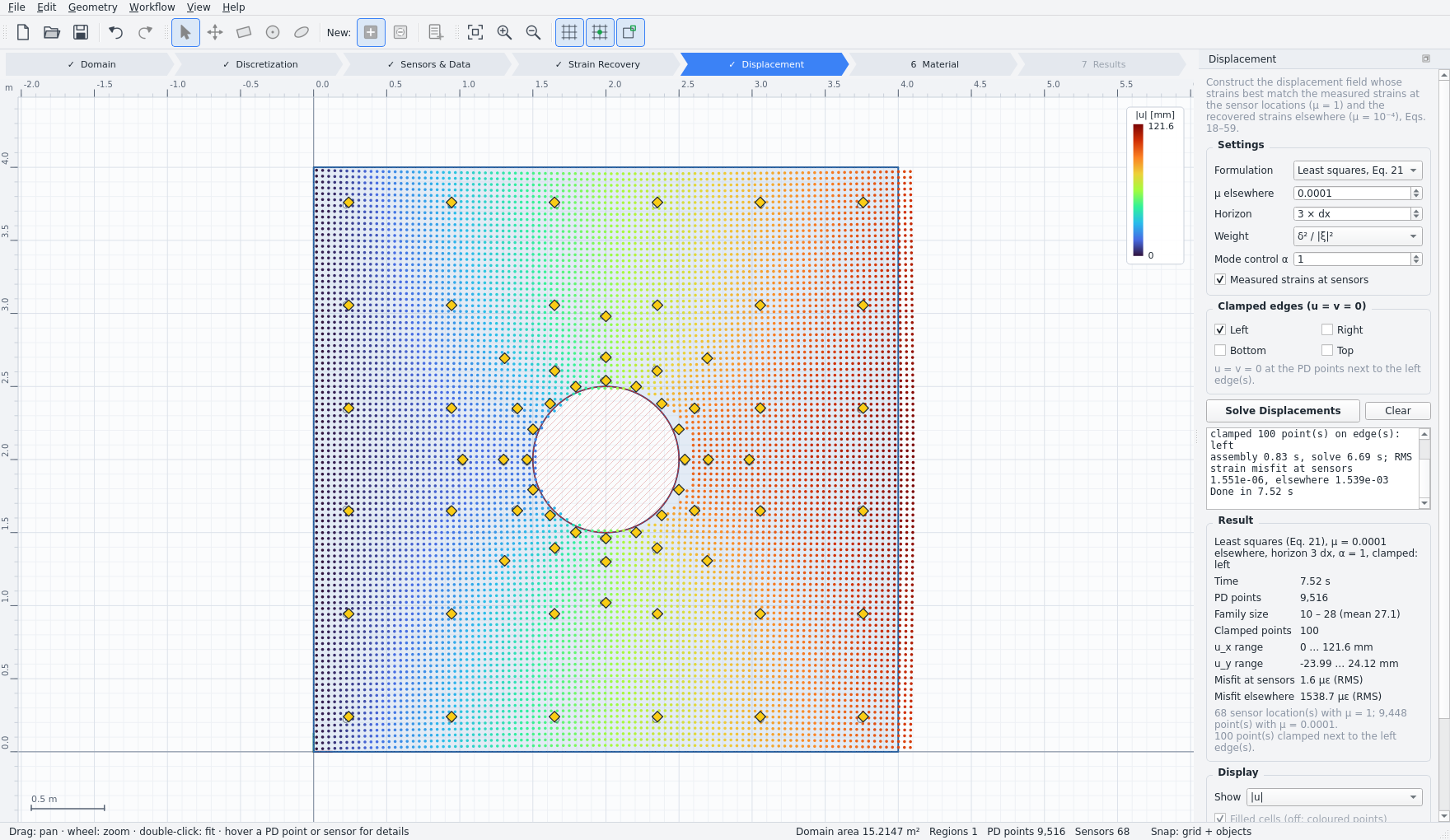 Step 5. The deformed shape at automatic magnification, coloured by |u| — reconstructed from strain data alone, with no model of the part.
Features
- Step-by-step graphical user interface with an interactive result canvas
- Works with any sensor layout — no regular grid or minimum count required
- Analytic geometry: rotatable rectangles, circles and ellipses, as parts or cut-outs
- Grid, quadtree-refined, body-fitted ring, scattered and imported discretizations
- Automatic unit and shear-convention handling (strain, µε, %, tensor or engineering)
- Native C++/OpenMP solver with a NumPy reference implementation as cross-check
- Interactive pan and zoom, hover read-out of every point's values
- Deformed-shape view with automatic magnification
- Unlimited undo and redo with a history panel
- Project files that store geometry, points, sensors and every result
- Export of points, strains, displacements and stresses to CSV
- Open Python platform — scriptable, with a standalone command-line solver
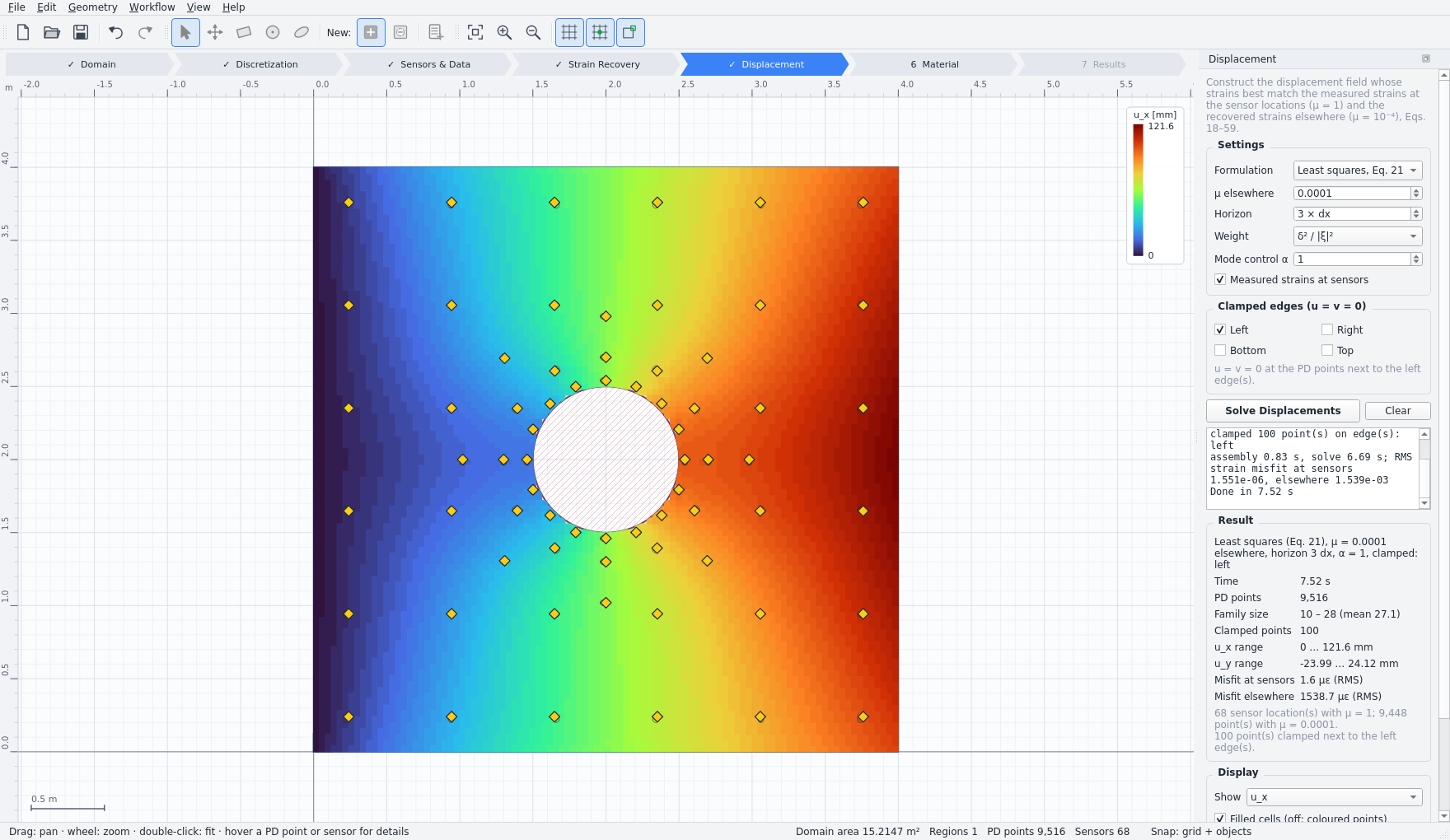 Step 5. Horizontal displacement ux, constructed from the strain field by least squares.
Capabilities
- Full strain field εxx, εyy, γxy from sparse point measurements
- Continuous displacement field without a finite element model of the part
- Stresses σxx, σyy, τxy and von Mises from the identified law
- Young's modulus E and Poisson's ratio ν from the measured load resultant alone
- Geometry-aware families that never reach through a hole, notch or slit
- Zero-energy-mode control for smooth, noise-robust displacement fields
- Body-fitted ring meshes around circular and elliptical cut-outs
- Diagnostics: family size, horizon and noise amplification at every point
- Consistency check that flags an unreliable reconstruction without a reference
- Export of every field for downstream fatigue, fracture or certification work
Material Identification
With the strain field reconstructed, the elastic constants follow from the principle of virtual work. For every admissible virtual field — zero on the supported edge, where the reaction is unknown, and rigid on the loaded edge, so that only the measured resultant does work — the internal and external virtual work must balance. Each field gives one linear equation in the plane stiffnesses, and six polynomial fields are solved by least squares. Nothing but the strain field, the measured load and the thickness enters the calculation.
Because the virtual strains are PDDO derivatives taken with the same operator that differentiates the reconstruction, the quadratic virtual fields are differentiated exactly. The six fields would agree perfectly on a field in equilibrium, so their spread is reported as a consistency measure — a warning that the reconstruction is unreliable, available without any reference solution to compare against. An optimised-virtual-field mode instead minimises sensitivity to strain noise and reports the resulting noise amplification directly.
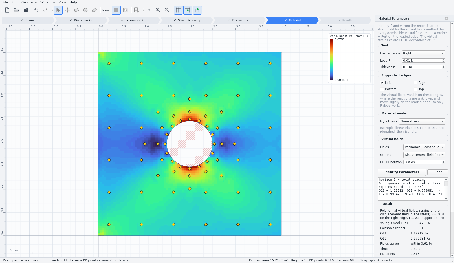 Step 6. Von Mises stress from the identified constants. Here E = 0.9995 and ν = 0.3306 against true values of 1 and 1/3, with the six virtual fields agreeing within 0.61 %.
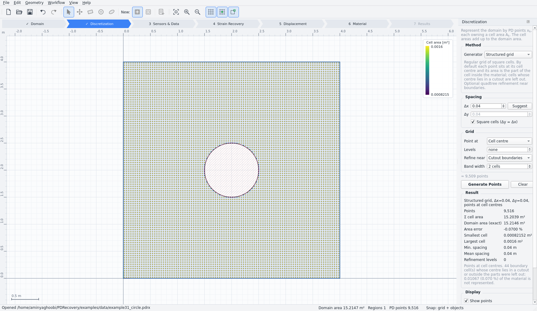 Step 2. Peridynamic points coloured by cell area; cells are trimmed exactly to the curved cut-out.
Validated Accuracy
The reconstruction is validated against finite element reference solutions for a square plate under tension with a circular hole, an inclined elliptical hole, and a slit. Errors below are the relative RMS over every peridynamic point, from 42 to 82 sensors on grids of 9,500 to 9,900 points.
- Circular cut-out, 68 sensors: strains 2.9 to 6.2 %, displacements 0.8 and 3.8 %
- Elliptical cut-out, 82 sensors: strains 3.6 to 5.6 %, displacements 1.1 and 2.1 %
- Slit, 42 sensors: strains 5.1 to 8.0 %, displacements 4.5 and 4.3 %
- Identified constants: E within 0.1 to 8.2 % and ν within 0.8 to 12.2 % of the true values
- Native and reference solvers agree to machine precision on every case
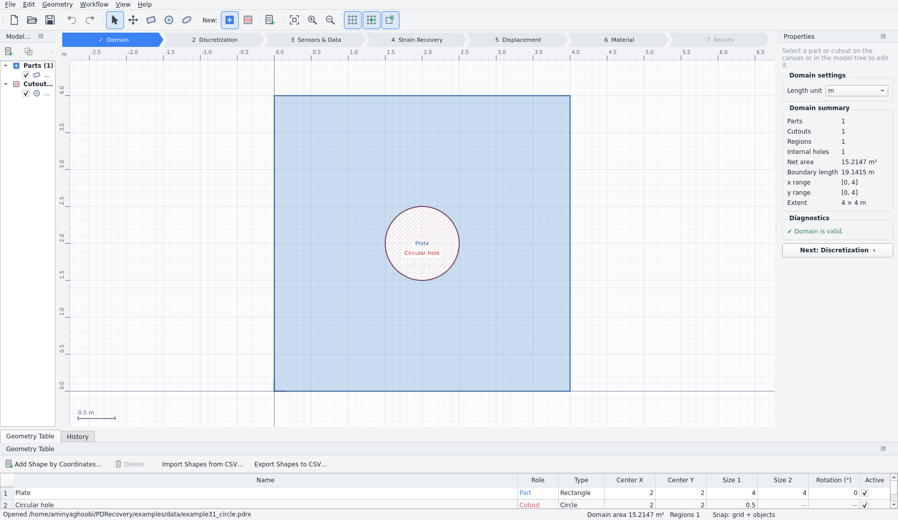 Step 1. The domain is built from analytic primitives as parts and cut-outs, with live diagnostics for net area, boundary length, regions and holes.
Who Is It For
- Structural health monitoring — turn a permanent gauge array into a full-field picture of the structure
- Test engineers — recover the fields between the gauges on a component or full-scale test article
- Certification and airworthiness — evidence of strain and stress where no gauge could be placed
- Materials characterisation — identify elastic constants from a single heterogeneous test
- Digital twins — feed a measured, continuous field into a model instead of point readings
- Fatigue and fracture assessment — measured stress fields at the critical detail
All Products