1Getting Started
PDDIC measures full-field displacement and strain from experimental images, and locates cracks automatically. You supply a reference image and one or more deformed images; PDDIC tracks the displacement between them, computes the strain field, and flags regions where the deformation is no longer physically compatible — which is where damage is.
Everything is done through the graphical interface. There is nothing to script and nothing to compile.
1.1System Requirements
| Requirement | Detail |
|---|---|
| Operating system | Windows 10 or 11, 64-bit. |
| Disk space | Approximately 1 GB for the installation, plus room for your results. |
| RAM | 8 GB minimum; 16 GB recommended for large images or fine grids. |
| Display | 1280 × 800 or larger. |
| Internet | Required once to activate. After that PDDIC renews its license quietly in the background, and keeps working offline between renewals. An offline activation path is available for air-gapped machines. |
| Administrator rights | Required to install, but not to run. |
1.2Installing PDDIC
- Download PDDIC-Setup-1.0.0.exe from the link in your purchase email.
- Double-click the installer. Windows will ask for administrator permission — accept it.
- Read and accept the End User License Agreement.
- Choose the installation folder, or accept the default (C:\Program Files\PDDIC).
- Optionally tick Create a desktop shortcut.
- Click Install, then Finish.
PDDIC appears in the Start menu under PDDIC. Launch it from there, or from the desktop shortcut if you created one.
1.3Activating Your License
The first time you launch PDDIC, the Activate PDDIC window opens. PDDIC will not run until it is activated.
Activate online (normal method)
- Open the Activate Online tab.
- Type or paste the license key from your purchase email. It has the form ABCDE-FGHJK-LMNPQ-RSTUV. Lower-case letters are converted to upper-case as you type, so you can paste it in whatever form you received it.
- Click Activate.
PDDIC contacts the license server, claims one seat on your license for this machine, and opens the main window. This takes a few seconds.
Activate offline (air-gapped machines)
If the computer running PDDIC has no internet access:
- Open the Offline Activation tab.
- Enter your license key.
- Click Save Request File… and save the .json request somewhere you can reach it.
- Email that file to licensing@gertechnologies.com from any machine with internet access.
- You will receive a lease file in reply. Copy it to the offline machine.
- Return to the Offline Activation tab, click Import Lease File…, and select the file you were sent.
PDDIC starts as soon as the lease is imported.
1.4Managing Your License
Open File ▸ License… at any time to see the current status:
| Field | What it shows |
|---|---|
| Status | Active, or the reason PDDIC is not licensed. |
| License key | The key this machine is activated with. |
| Registered to | The email address the license was issued to. |
| Organisation | Your organisation, if one was recorded. |
| Seats on license | How many machines your license permits in total. |
| Subscription expires | The date your subscription ends. |
| Current lease expires | The date this machine's lease runs out, and the days remaining. |
| Features | Which capabilities your license includes (all for a full license). |
How the lease works
After activation PDDIC holds a 14-day lease. Once the lease is a week old, PDDIC renews it quietly in the background the next time it starts with an internet connection — you never see this happen. If the server cannot be reached, your existing lease keeps working until it expires, so a network outage never stops your work mid-session.
Moving PDDIC to a different computer
Each activation uses one seat. To free that seat, click Deactivate This Machine in the License window and confirm. PDDIC stops working on that computer, and you can activate the same key on the replacement machine.
1.5The Main Window
| Area | What it is |
|---|---|
| Step panel (left) | The eight analysis steps. Move through them with the Back and Next buttons at the bottom. Each step has a ? button that opens help for that step. |
| Canvas (right) | Shows the reference image and every result field. Supports pan, zoom, and drawing of lines and boxes for post-processing. |
| Tab bar (above canvas) | Images · Tracking Results · PD Regression Results · FD Strain Results · PD Differentiation Results · Crack Detection Results. |
| Canvas toolbar | Zoom In · Zoom Out · Move · Home · Save PNG · Line Plot · Box Plot · Settings · Save Results. |
| Status and progress | Appear at the bottom of the step panel while a solver is running. |
1.6Where Results Are Saved
PDDIC writes its results to a per-user data folder, not to the installation directory. Open File ▸ Open Output Folder to go straight there in Windows Explorer.
Keeping results out of C:\Program Files means PDDIC never needs administrator rights to run, and your results survive an uninstall or upgrade untouched.
1.7Getting Help
The Help menu contains:
| Menu item | What it does |
|---|---|
| User Manual | Opens this manual at https://www.gertechnologies.com/PDDIC/userManual. |
| About PDDIC | Version number and a short description of the software. |
| Contact | Starts an email to admin@gertechnologies.com in your mail client. |
2Workflow — Step by Step
PDDIC works through eight steps. Steps 1–3 define the geometry, Steps 4–7 run the solvers, and Step 8 detects cracks. Run them in order — each step consumes the previous one's output. Step 6 (FD Strain) is the one exception: it is optional and feeds nothing downstream.
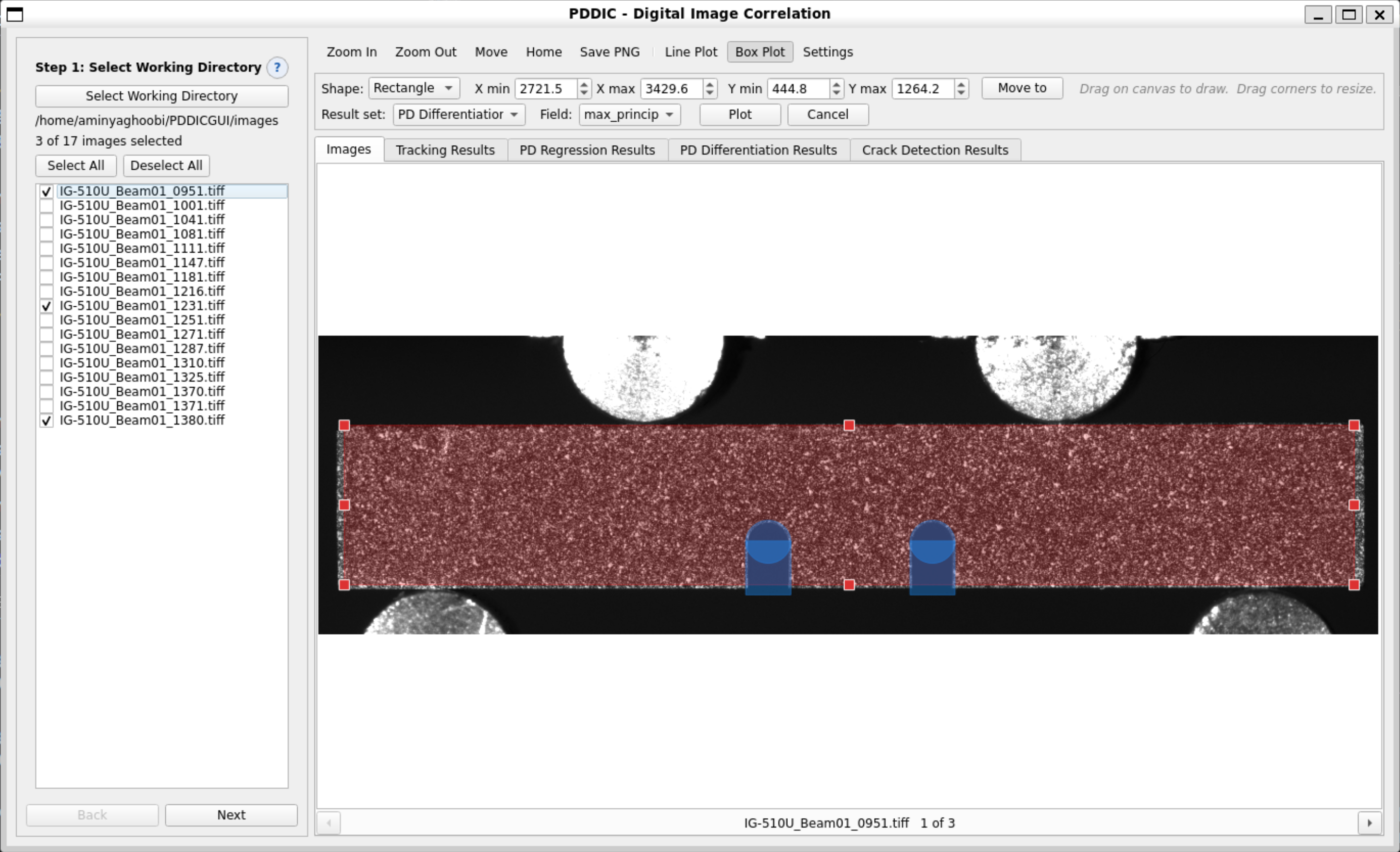
2.1Step 1 — Select Working Directory
Choose the folder holding your reference and deformed images. TIF, PNG, JPG, and BMP are all recognised.
Procedure
- Click Browse and select the folder.
- Every recognised image appears in the list with a checkbox.
- Tick each image you want to analyse. The first ticked image is the reference (undeformed) state; the rest are deformed states, analysed in list order.
- Click Next.
Use Select All / Deselect All to work through long sequences quickly. The reference image appears in the Images tab as soon as it is selected.
2.2Step 2 — Domain Selection
Define the rectangular region of interest. Everything downstream — tracking, regression, differentiation, crack detection — is confined to this region.
Procedure
- Interactively: drag a rectangle directly on the reference image. The coordinate fields update as you drag.
- By typing: enter values in xmin, xmax, ymin, ymax, then click Apply Domain.
| Parameter | Description |
|---|---|
| xmin / xmax | Left and right boundaries of the domain, in pixels. |
| ymin / ymax | Top and bottom boundaries of the domain, in pixels. |
Keep the domain inside the specimen. Including background or grip hardware wastes computation and adds points that cannot be tracked.
2.3Step 3 — Cut-outs
Cut-outs are exclusion zones — holes, notches, pre-existing voids, grip regions. Points inside a cut-out are excluded from tracking, and also from the regression neighbourhood of nearby points, so displacement is never blended across a physical boundary.
Adding a cut-out
- Choose Rectangle or Circle (an ellipse fitted to the bounding box).
- Click Add Cut-out, then drag on the image — or type the bounding box coordinates and click Add Cut-out.
- Drag the corner handles to fine-tune the shape.
Managing cut-outs
| Action | What it does |
|---|---|
| Edit (pencil icon) | Load the cut-out into the form, adjust the values, then click Save. |
| Clone (copy icon) | Duplicate the cut-out at the same position and size. |
| Delete (trash icon) | Permanently remove the cut-out. |
You can define as many cut-outs as you need, mixing rectangles and circles freely. Their geometry carries through to every later step automatically.
2.4Step 4 — Subset Tracking (DIC)
Tracking measures how far small image patches move between the reference image and each deformed image. The result is a sparse field of displacement vectors (U, V).
Procedure
- Set Subset size and Min point distance — these are the two parameters that matter most.
- Adjust anything under Advanced Settings only if you need to.
- Click Run Tracking. A progress bar and status message track the run.
- Results appear in the Tracking Results tab. Choose U or V from the drop-down to view horizontal or vertical displacement.
| Parameter | Description |
|---|---|
| Subset size (odd px) | Side length of the correlation patch. Must be odd. Larger subsets are more stable on weak texture but blur fine detail. Typical range 15–51 px. Default: 21. |
| Min point distance (px) | Minimum spacing between tracked points. Controls how dense the point cloud is. Default: 10. |
Advanced Settings
The remaining parameters are collapsed behind the Advanced Settings toggle, which starts closed. Click it to expand the section, click it again to fold it away. The defaults suit most experiments — open this section when the defaults are not working, not before.
| Parameter | Description |
|---|---|
| Search radius (px) | Largest displacement searched in the deformed image. Must exceed your biggest expected displacement. Default: 30. |
| Correlation threshold | Minimum correlation score (0–1) for a match to be accepted. Lower keeps more points but admits more noise. Default: 0.75. |
| Min texture std-dev | Rejects flat, featureless subsets below this grey-level standard deviation. Default: 5.0. |
| Median filter size (odd) | Median filter applied to the displacement results. Odd integer; 0 or 1 disables it. Default: 3. |
| Gaussian sigma | Optional Gaussian smoothing of the results, applied after the median filter. 0 disables it. Default: 0. |
| Max points | Hard cap on tracked points per image. Default: 5000. |
| Failure streak limit | Stops seeding after this many consecutive failed placements. Default: 5000. |
| Random seed | Seed for reproducible point placement. Change it to get a different distribution from identical settings. Default: 42. |
2.5Step 5 — PD Regression
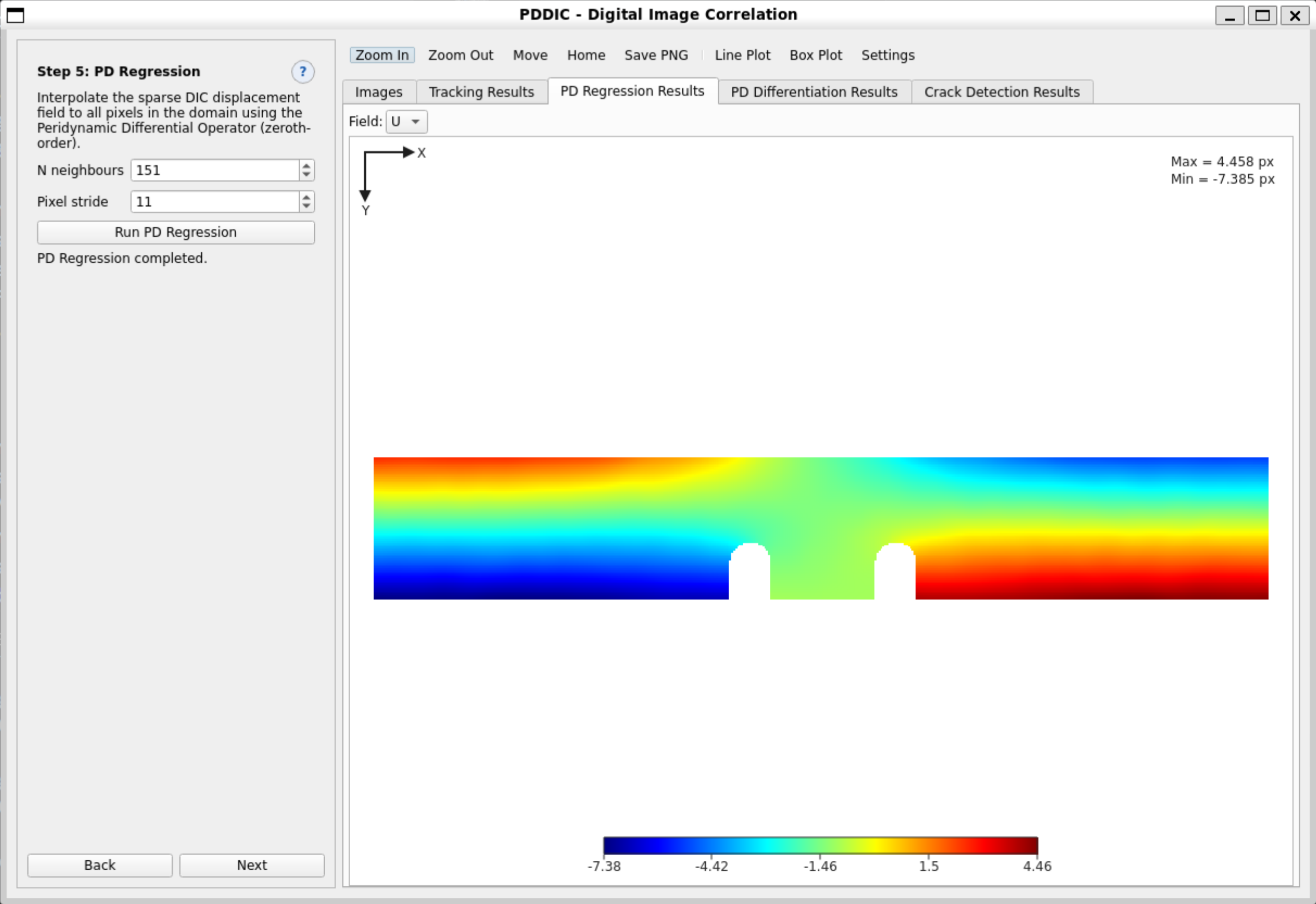
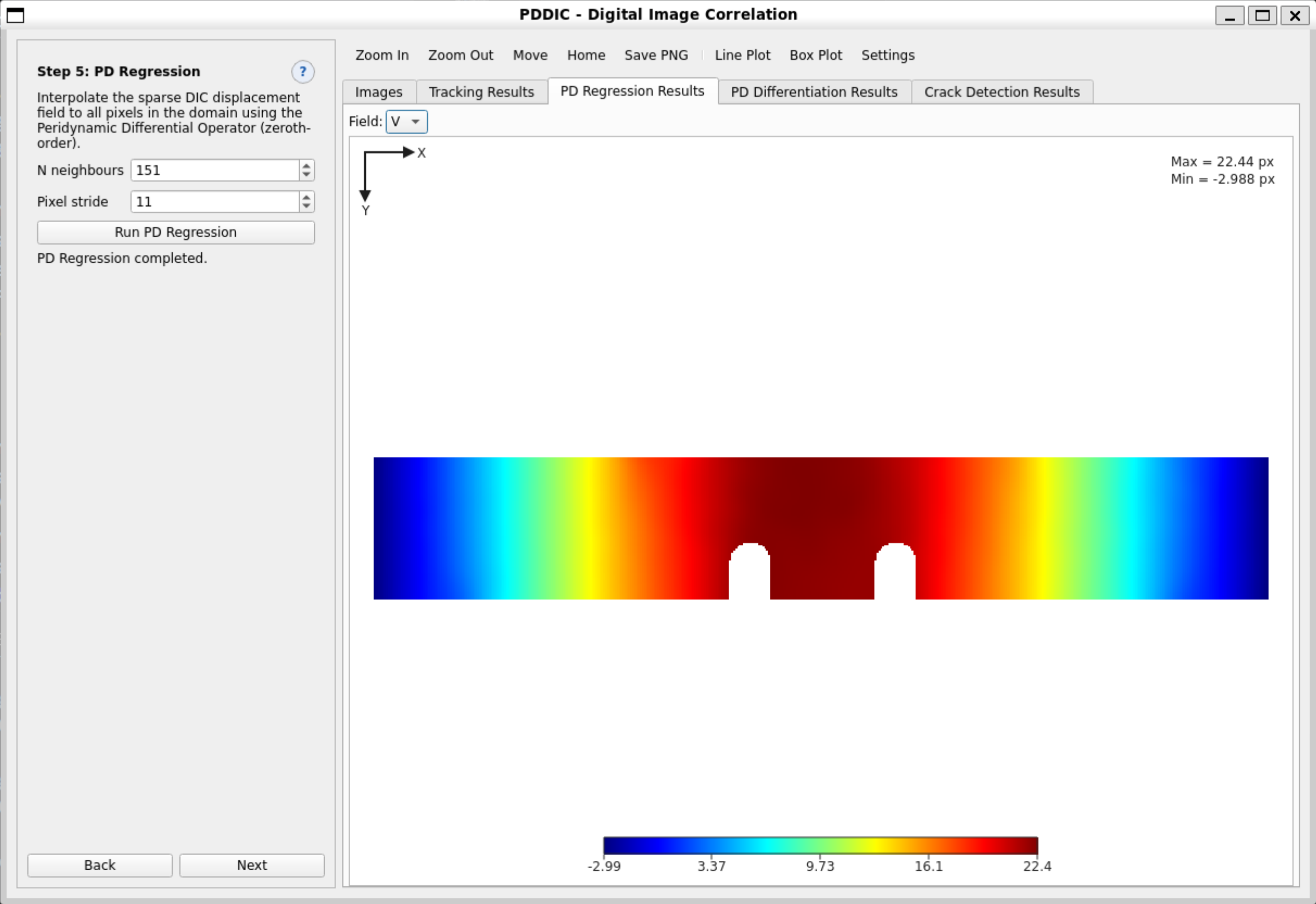
Regression spreads the sparse tracked displacements onto a dense, regular grid using the zeroth-order Peridynamic Differential Operator. The output is a smooth displacement map covering the whole domain.
Procedure
- Set the parameters below.
- Click Run PD Regression. The solver runs in the background.
- The dense U and V fields appear in the PD Regression Results tab.
| Parameter | Description |
|---|---|
| N neighbours | How many nearby tracked points contribute to each output point. Larger values smooth more, but can wash out sharp gradients. Typical range 10–60. Default: 51. |
| Pixel stride | Output spacing in pixels. 1 = every pixel (finest, slowest); 4 = one point per 4×4 block (coarser, much faster). Default: 1. |
2.6Step 6 — FD Strain (Optional Preview)
A fast strain estimate computed by finite differences on the regression grid. Treat it as a preview — Step 7 produces the strain fields you should actually report.
| Parameter | Description |
|---|---|
| Smooth σ (px) | Gaussian pre-smoothing of U and V before differentiation. 0 disables it. Larger values suppress noise but blur sharp features. Default: 5.0. |
Output fields
| Field | What it is |
|---|---|
| strain_x | ∂U/∂x — normal strain in the horizontal direction. |
| strain_y | ∂V/∂y — normal strain in the vertical direction. |
| shear_xy | ½(∂U/∂y + ∂V/∂x) — engineering shear strain. |
2.7Step 7 — PD Differentiation
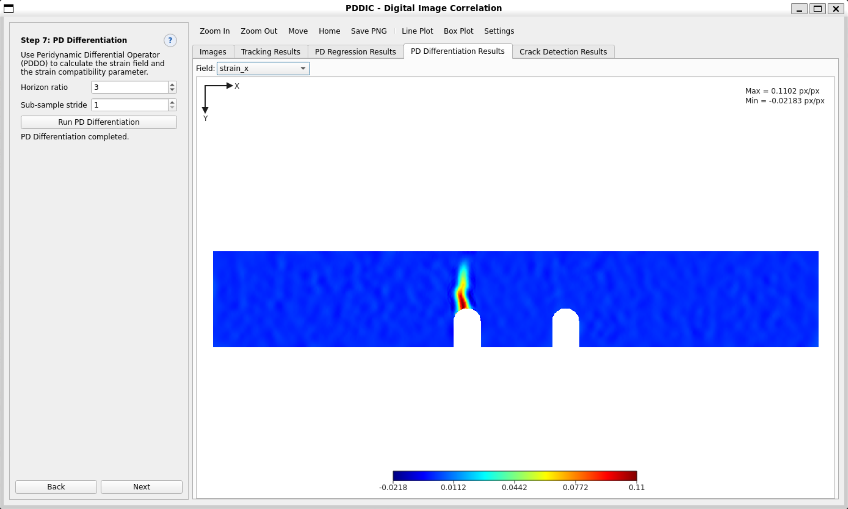
The main strain analysis. The first-order PDDO differentiates the dense displacement field from Step 5, producing the full strain field plus the compatibility residual and Damage Confidence Factor that Step 8 needs.
Procedure
- Set the parameters below.
- Click Run PD Differentiation. The solver runs in the background; a status message confirms completion.
- Results appear in the PD Differentiation Results tab.
| Parameter | Description |
|---|---|
| Horizon ratio | Size of the differentiation neighbourhood, as a multiple of the point spacing. Larger gives smoother strain; smaller resolves finer gradients. Range 1–5, typical 2–4. Default: 3. |
| Sub-sample stride | Thins the regression grid before differentiating. 1 = use every point; 2 = every other point. Raise it to cut computation time. Default: 1. |
Output fields
| Field | What it is |
|---|---|
| U, V | Displacement components. |
| strain_x | Normal strain εx = ∂U/∂x. |
| strain_y | Normal strain εy = ∂V/∂y. |
| strain_xy | Shear strain εxy = ½(∂U/∂y + ∂V/∂x). |
| max_principal_strain | Maximum principal strain at each point. |
2.8Step 8 — Crack Detection
Step 8 finds cracks from the compatibility residual computed in Step 7. It needs no prior knowledge of where the crack is, which way it runs, or how long it is.
What happens when you click Detect Cracks
- Boundary masking — points within 4× the point spacing of the domain edge or any cut-out are dropped, since boundaries produce compatibility artefacts that look like damage.
- Damage confidence — the residuals of the remaining interior points are standardised into a two-tailed p-value. A point with a large residual gets a low CDF, meaning high damage probability.
- Candidate selection — points with CDF at or below the threshold are flagged and displayed.
- Crack path fitting — clustering isolates the dense crack region from scattered noise, the principal crack direction is identified, and a smooth curve is fitted along it to predict the continuous crack path.
| Parameter | Description |
|---|---|
| CDF threshold | Cut-off between 0.0 and 1.0. Points at or below it are flagged as crack candidates. Lower flags more; higher is more conservative. Default: 0.75. |
Output views
| View | What it shows |
|---|---|
| compatibility | Compatibility residual across the interior domain. Large values mean kinematic discontinuity. |
| cdf | Damage Confidence Factor. Low values mean likely damage. |
| remaining_points | The flagged crack candidates, with the mask boundary drawn in. |
| detected_crack | The analysis region boundaries. |
The black lines on the last two views mark the masked region: the domain shrunk by 4× the point spacing, and each cut-out enlarged by the same margin.
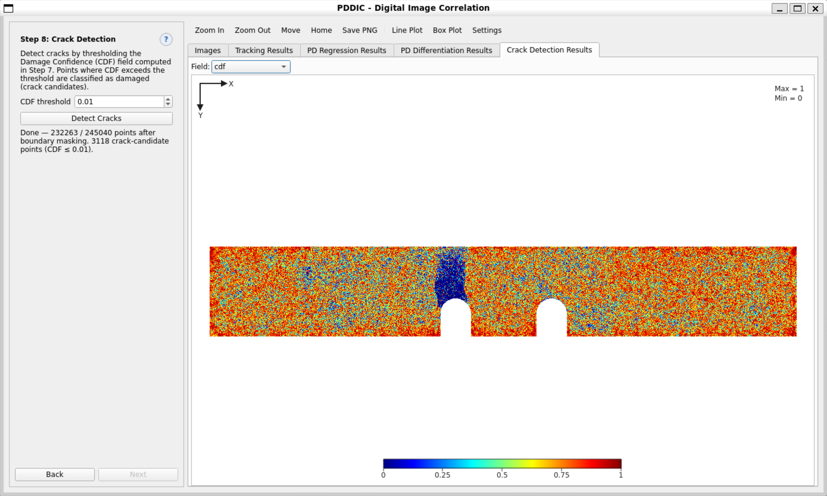
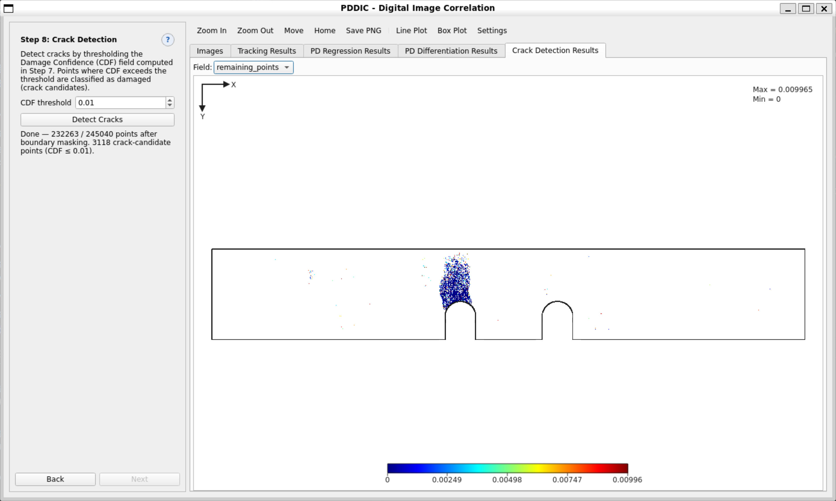
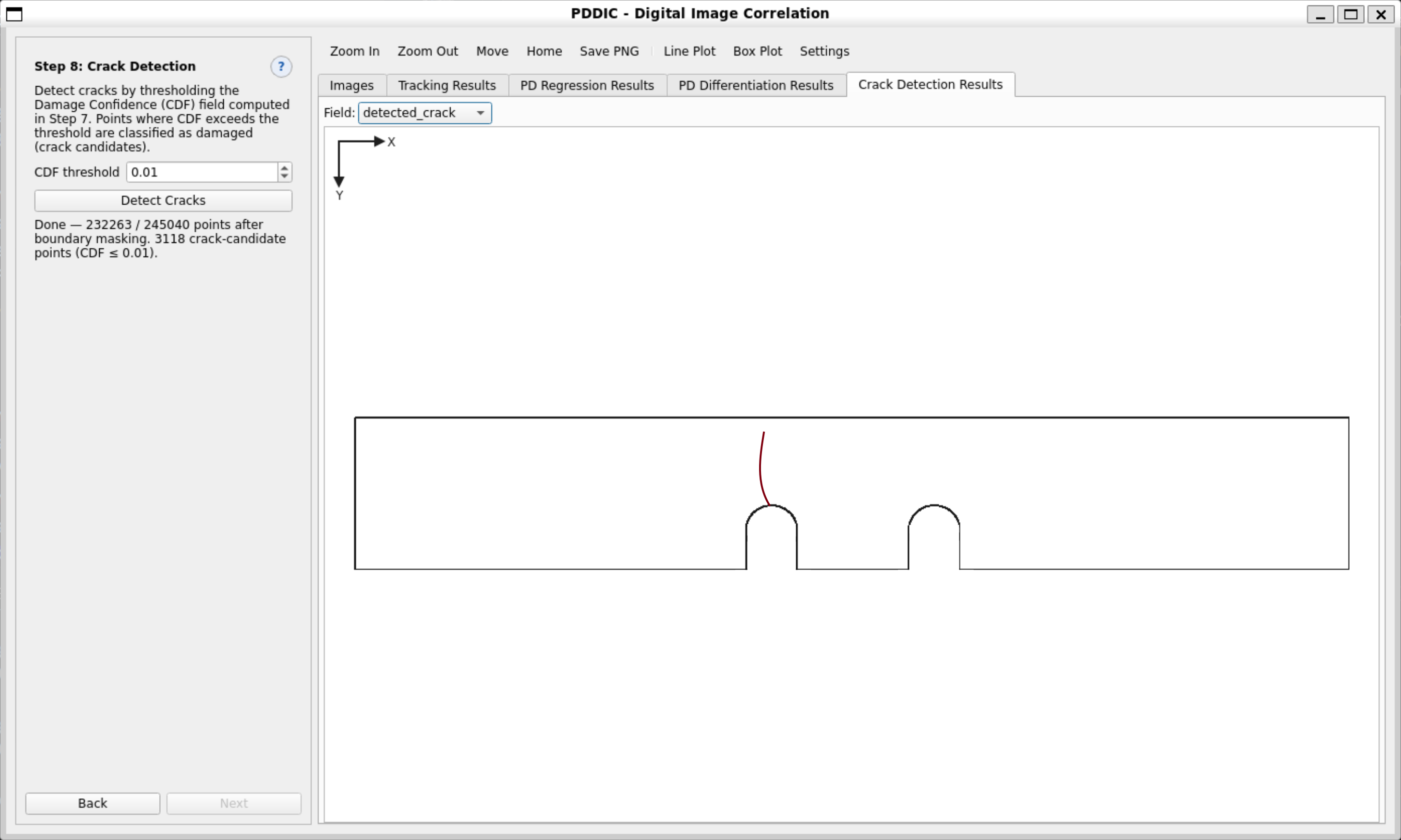
3Post-Processing Tools
All of these live on the canvas toolbar and act on whichever result tab is currently open.
3.1Canvas Navigation
| Control | What it does |
|---|---|
| Zoom In / Zoom Out | Magnify or shrink by a fixed step. |
| Scroll wheel | Zoom continuously at the cursor position. |
| Move | Toggle pan mode, then drag to pan the canvas. |
| Home | Reset zoom and pan to fit the full result in the viewport. |
| XY arrow helper | The small indicator in the bottom-left corner showing the image x/y axis directions. |
3.2Plot Settings
Click Settings on the toolbar. Changes apply immediately to every result canvas.
Color scheme
| Colormap | Description |
|---|---|
| Jet | Classic blue–cyan–green–yellow–red rainbow colormap (default). |
| Jet_m | Jet truncated to its central 75% — less saturated at the extremes. |
| Viridis | Perceptually uniform blue–green–yellow colormap. Best for publication. |
| Coolwarm | Diverging blue–white–red colormap. Best for signed fields such as displacement. |
Number of colors
| Mode | Description |
|---|---|
| Continuous | Smooth gradient colorbar (default). |
| Discrete | Quantise the colorbar into a fixed number of bands (2–256). |
Color range
| Mode | Description |
|---|---|
| Automatic | Spans the current field's minimum and maximum (default). |
| Manual | Takes explicit vmin and vmax values. Use this to compare several images on one fixed scale, or to highlight a specific value range. |
Unit
Displacement fields can be displayed in physical units instead of pixels. Choose the unit and enter the conversion factor.
| Unit | Description |
|---|---|
| px (default) | Display in pixels — no conversion applied. |
| μm | Micrometres. Enter the number of pixels per micrometre. |
| mm | Millimetres. Enter the number of pixels per millimetre. |
| cm | Centimetres. Enter the number of pixels per centimetre. |
| m | Metres. Enter the number of pixels per metre. |
Once you pick a unit, it propagates everywhere: colorbar ticks, the min/max overlay labels, Line Plot and Box Plot axes, and the coordinate input fields.
Coordinate axes
| Option | Description |
|---|---|
| Show | Display X/Y axis labels, tick marks, and a grid on the result canvas. |
| Hide | Hide the coordinate axes (default). The XY arrow helper remains visible. |
3.3Line Plot
Extracts field values along a straight line you draw — ideal for a profile across a crack tip or along a gauge length.
Procedure
- Click the Line Plot toggle. A coordinate bar appears below the toolbar.
- Click once on the canvas to set Point 1 (P1), then click again to set Point 2 (P2). White handles mark the endpoints.
- Drag the handles to adjust, or type coordinates into the P1/P2 fields and click Move to.
- Choose the Result set and Field.
- Optionally tick Normalize Y to divide values by their maximum absolute value.
- Click Plot.
Line Profile window controls
| Control | What it does |
|---|---|
| Result set | Switch between Tracking Results, PD Regression, and PD Differentiation without redrawing the line. |
| X axis | Distance along the line, X coordinate, Y coordinate, or (X, Y) coordinate pairs. |
| Field | Which displacement or strain component to plot on the Y axis. |
| Normalize Y | Divide Y values by max|field| to normalise the profile to [−1, 1]. |
3.4Box Plot
Extracts every data point inside a region you draw and shows their spatial distribution as a colour-mapped scatter plot — useful for inspecting a notch tip or a specific gauge section statistically.
Procedure
- Click the Box Plot toggle. A coordinate bar appears below the toolbar.
- Select the region shape: Rectangle or Circle.
- Drag on the canvas to draw the region, or type the bounds and click Move to.
- Choose the Result set and Field.
- Click Plot.
The scatter plot uses the colormap and unit from Plot Settings, and updates live as you drag the region's corner handles.
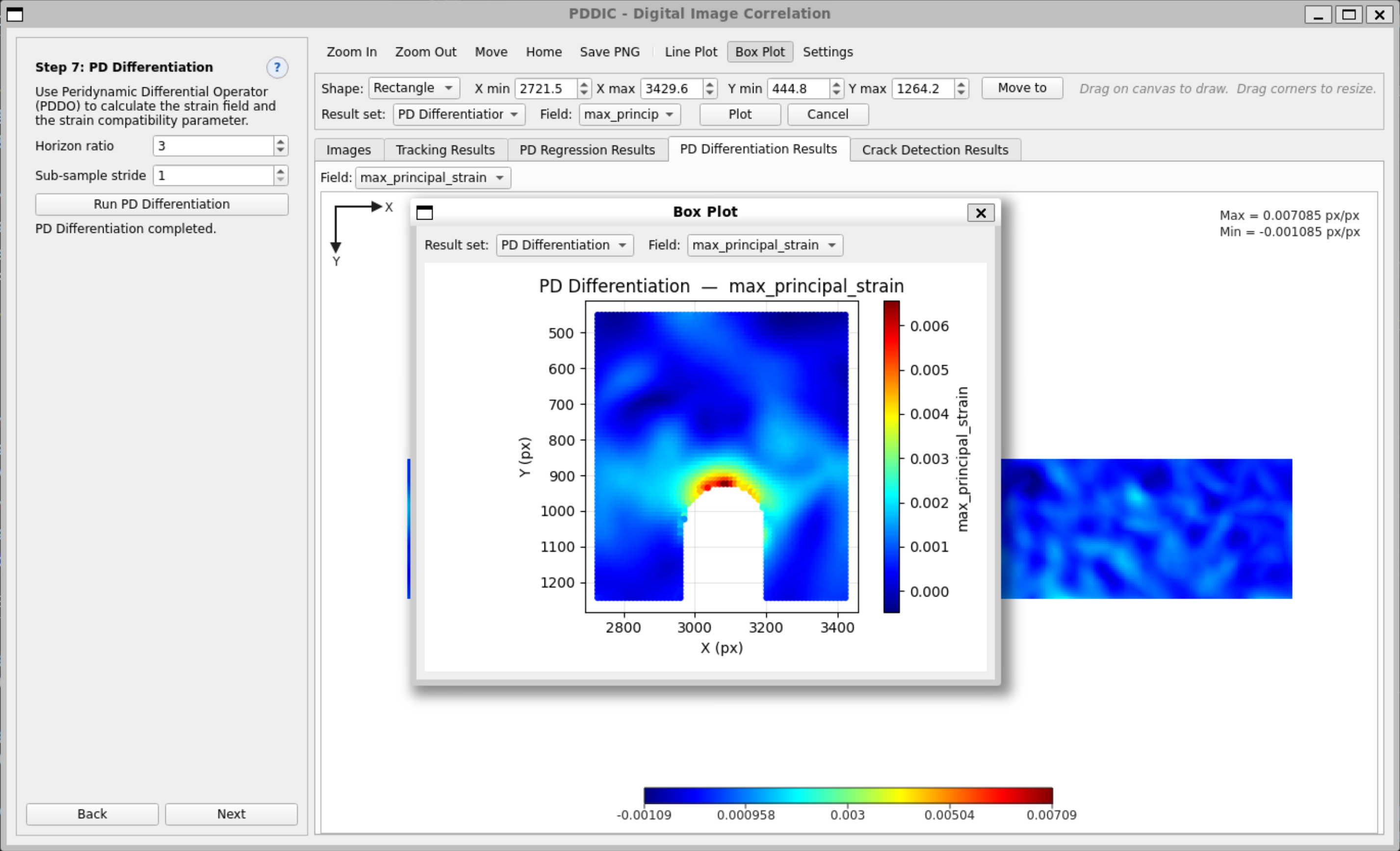
3.5Save PNG
Exports the current canvas view — colorbar overlay and axis helper included — as a PNG image file. A file-save dialog prompts for the output path.
3.6Save Results
Exports numerical data to a plain text file. A dialog lists the datasets you have computed; pick one.
| Dataset | Columns |
|---|---|
| Tracking Results | Columns: x y U V correlation One row per tracked point. |
| PD Regression Results | Columns: x y U V One row per output grid point. |
| PD Differentiation Results | Columns: x y U V strain_x strain_y strain_xy max_principal_strain compatibility cdf One row per PDDO point. |
The file opens with two comment lines describing its content, then the point count, then one row per point. Coordinates and displacements are in pixels; strains are dimensionless.
4Tips and Troubleshooting
4.1Preparing Your Images
- Use a high-contrast random speckle pattern. Speckles should span roughly 3–5 pixels so that each subset contains several of them.
- Minimise out-of-plane motion, rigid-body rotation, and lighting changes between frames.
- 8-bit or 16-bit greyscale is ideal. Colour images are converted to greyscale internally.
- Keep image dimensions identical across the sequence.
4.2Choosing a Subset Size
- Too small: not enough texture, correlation scores fall, points get rejected.
- Too large: displacements are averaged over too wide an area and sharp gradients are lost.
- Rule of thumb: the subset should contain 3–5 speckles. Start at 21–31 px and adjust.
4.3Choosing a Horizon Ratio
- The default of 3 suits most work.
- Raise it to 4–5 when the strain field is noisy or the points are irregularly spread.
- Lower it to 2 when sharp gradients near a crack tip are being smoothed away.
4.4Choosing a CDF Threshold
- Start at the default 0.75.
- If real cracks are missed, lower it (try 0.5).
- If false positives appear away from the crack, raise it (try 0.85–0.90).
- Always inspect the CDF map before interpreting the result.
4.5Common Problems
| Problem | What to do |
|---|---|
| PDDIC will not start — "not activated" | Enter your license key when prompted. If you have lost it, email licensing@gertechnologies.com with your order details. |
| Activation fails — no seats available | Every seat on your license is in use. Free one with Deactivate This Machine on a computer you no longer need, or contact us to add seats. |
| Activation fails — server unreachable | Check your internet connection and any corporate firewall or proxy. If the machine has no internet at all, use the Offline Activation tab. |
| PDDIC stops working after weeks offline | The lease has expired. Connect to the internet and restart PDDIC; it renews itself automatically. |
| No tracked points found | Lower the Correlation threshold, raise the Subset size, or check your image quality and domain definition. |
| PD Differentiation fails on point count | Too many points. Raise the Pixel stride in Step 5 or the Sub-sample stride in Step 7. |
| Crack detection finds no candidates | Lower the CDF threshold, or confirm that Step 7 actually completed. |
| Line Plot or Box Plot shows nothing | Make sure the selected result set has been computed and that your line or box overlaps a region with data. |
5Glossary
| Term | Meaning |
|---|---|
| CDF (Damage Confidence Factor) | Statistical p-value of the compatibility residual. Low CDF = high damage probability. |
| Compatibility residual | How far the measured strain field departs from kinematic admissibility. Non-zero values indicate damage. |
| Cut-out | An exclusion zone (hole, notch, grip) omitted from analysis. |
| DIC (Digital Image Correlation) | Optical technique that tracks image patches between reference and deformed images to measure displacement. |
| Domain | The rectangular region of interest that all analysis is confined to. |
| Horizon | The peridynamic neighbourhood radius. Points within it interact in PDDO computations. |
| Horizon ratio | The horizon radius expressed as a multiple of the point spacing. |
| Lease | The time-limited authorisation PDDIC holds after activation. Renews automatically. |
| PDDO (Peridynamic Differential Operator) | Non-local, mesh-free operator for computing spatial derivatives. |
| PD Regression | Zeroth-order PDDO step that spreads sparse tracked displacements onto a dense grid (Step 5). |
| PD Differentiation | First-order PDDO step that computes strains and compatibility from the dense field (Step 7). |
| Pixel stride | Spacing between adjacent output points on the regression grid. |
| Seat | One machine's worth of your license allocation. |
| Subset | The square image patch centred on a tracked point. Its size is the primary resolution parameter. |
| U, V | Horizontal and vertical displacement components. |
PDDIC is licensed by Global Engineering Research and Technologies, LLC. Support: admin@gertechnologies.com · Licensing: licensing@gertechnologies.com