PDDO-MultiPhysics
Write the physics as equations. Solve it in 3D, coupled and in time, on a box or on any CAD part — with no mesh to build.
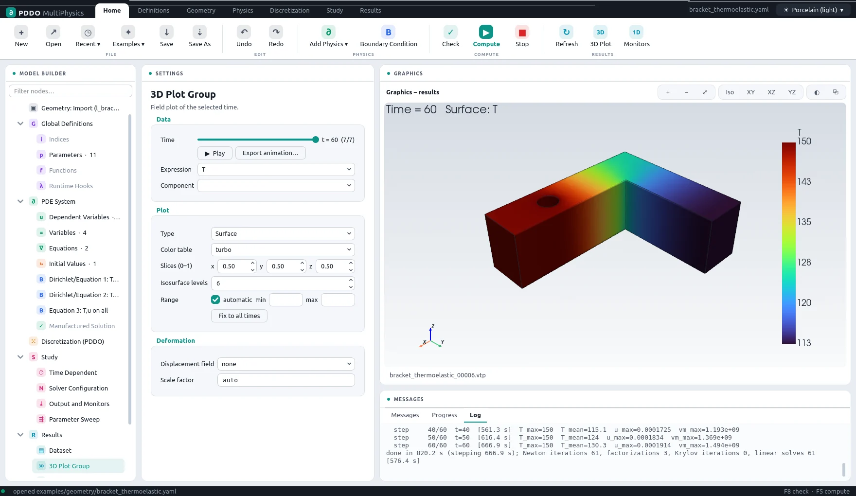 The interface. An aluminium bracket imported from STEP and heated through its bolt hole: the model builder, the settings of the selected node, the temperature on the part and the solver log.
About
PDDO-MultiPhysics solves transient, coupled, three-dimensional problems that you describe the way you would write them on paper: the unknown fields, the parameters, the constitutive relations, the partial differential equations, and the initial and boundary conditions. Heat conduction, elasticity, plasticity, viscoelasticity, fracture, phase separation, solidification, crystal growth, reaction–diffusion and chemo-mechanics all use the same few lines of a problem file — and so does the model nobody has written a solver for yet.
The engine is the Peridynamic Differential Operator (PDDO), a non-local, mesh-free way of computing derivatives of any order from a family of neighbouring points. The domain is a regular grid, or a point cloud that conforms to the surface of an imported STEP or STL part, with local refinement where the solution needs it. Every equation is differentiated symbolically, so Newton's method always has the exact Jacobian, and implicit, explicit and IMEX time schemes with error-controlled steps take the solution forward.
Models are set up, run and post-processed in a graphical interface laid out like the CAE tools engineers already know, or run from the command line and from Python.
Write the Physics, Not the Solver
A thermoelastic part takes two fields, four relations and two equations. The stress is written as lambda*tr(eps)*I + 2*G*eps - (3*lambda + 2*G)*alpha*(T - T0)*I, the equilibrium as div(sigma) = 0, and a traction-free face as dot(sigma, n) = [0, 0, 0] — nothing else. The engine turns them into discrete equations, works out which derivatives each one needs, chooses the order of the operators, and derives the exact Jacobian.
The language has the operators of continuum physics — gradient, divergence, Laplacian, biharmonic, curl, symmetric and deviatoric parts, traces, contractions, first and second time derivatives — and the functions of a scientific calculator. Parameters can be expressions, tables against time or temperature, data files, values per material, or a CALPHAD driving force computed from a thermodynamic database.
Scalar, vector and tensor fields; indexed fields for multigrain models; history fields with update rules for plasticity and fracture; local ODEs for viscoelasticity; Python hooks for anything that is not a PDE, such as nucleation.
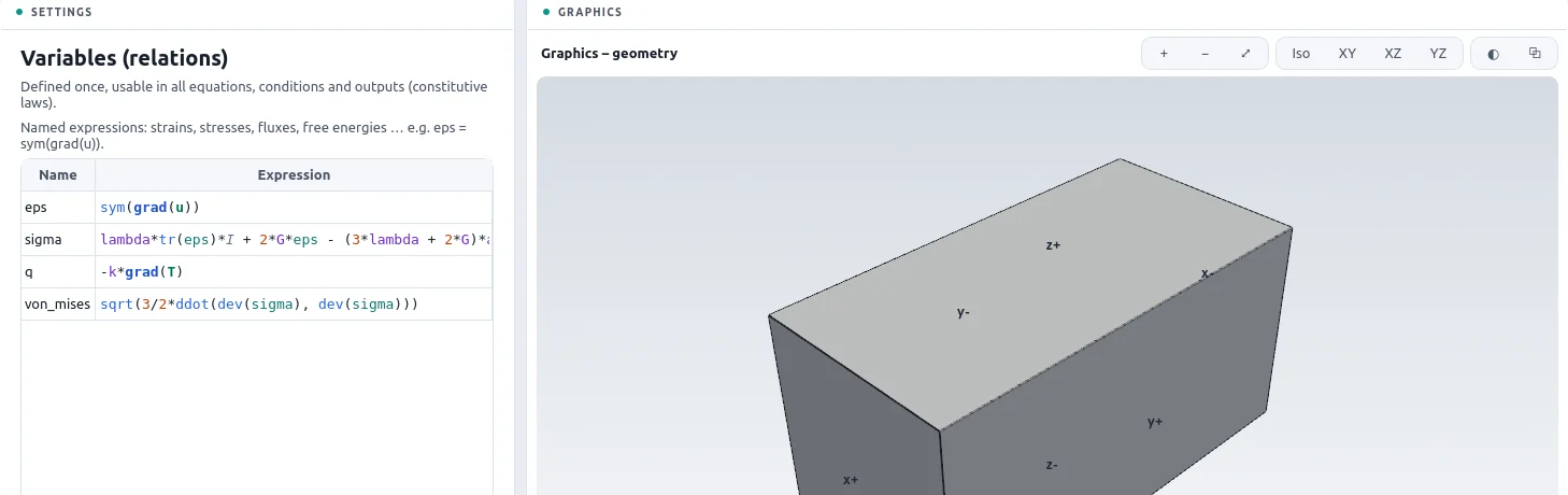 Constitutive relations. Strain, thermoelastic stress, heat flux and von Mises stress as typed in the Variables node, with syntax highlighting and undefined names underlined.
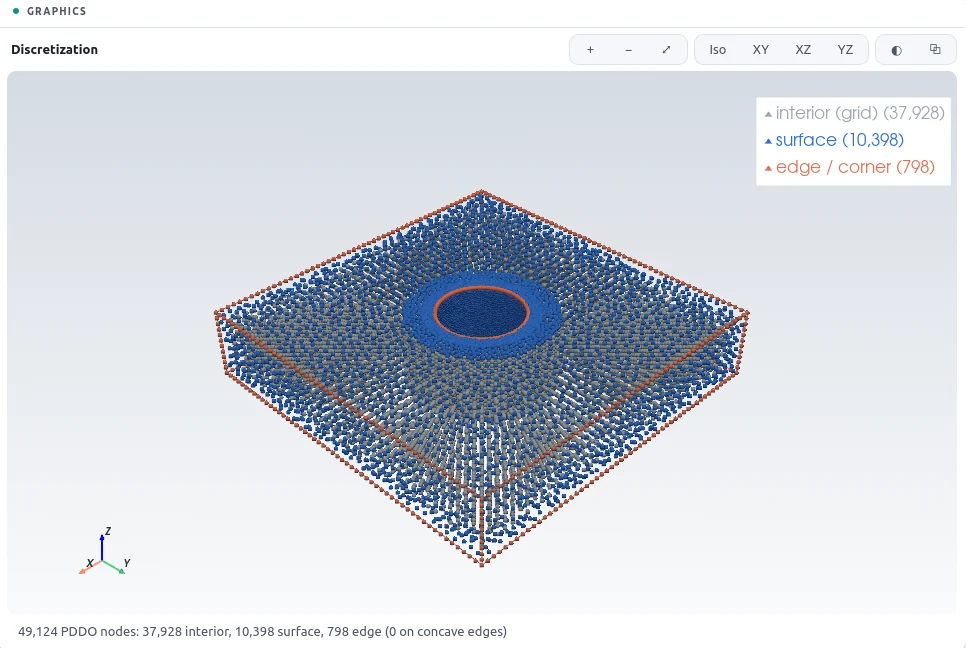 Local refinement. A STEP plate with 2.5 mm nodes in the plate and 0.625 mm nodes at the hole, graded smoothly in between.
Any Part, No Mesh
Import a STEP or STL file and choose a node spacing. The part is filled with a regular grid, nodes are placed exactly on its surface with the true normal, and its sharp edges get nodes of their own. Every boundary condition acts on the real CAD faces, which you rename and group in a table or pick with the mouse.
Refine around faces, inside boxes or spheres; the spacing grades smoothly and each level keeps a fast shared stencil. Build parts from several materials: list the bodies in order, give any parameter a value per region, and the interfaces between them carry continuity of the field and of its flux, read from the equations themselves.
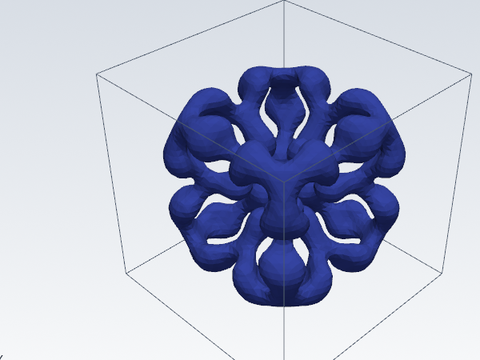
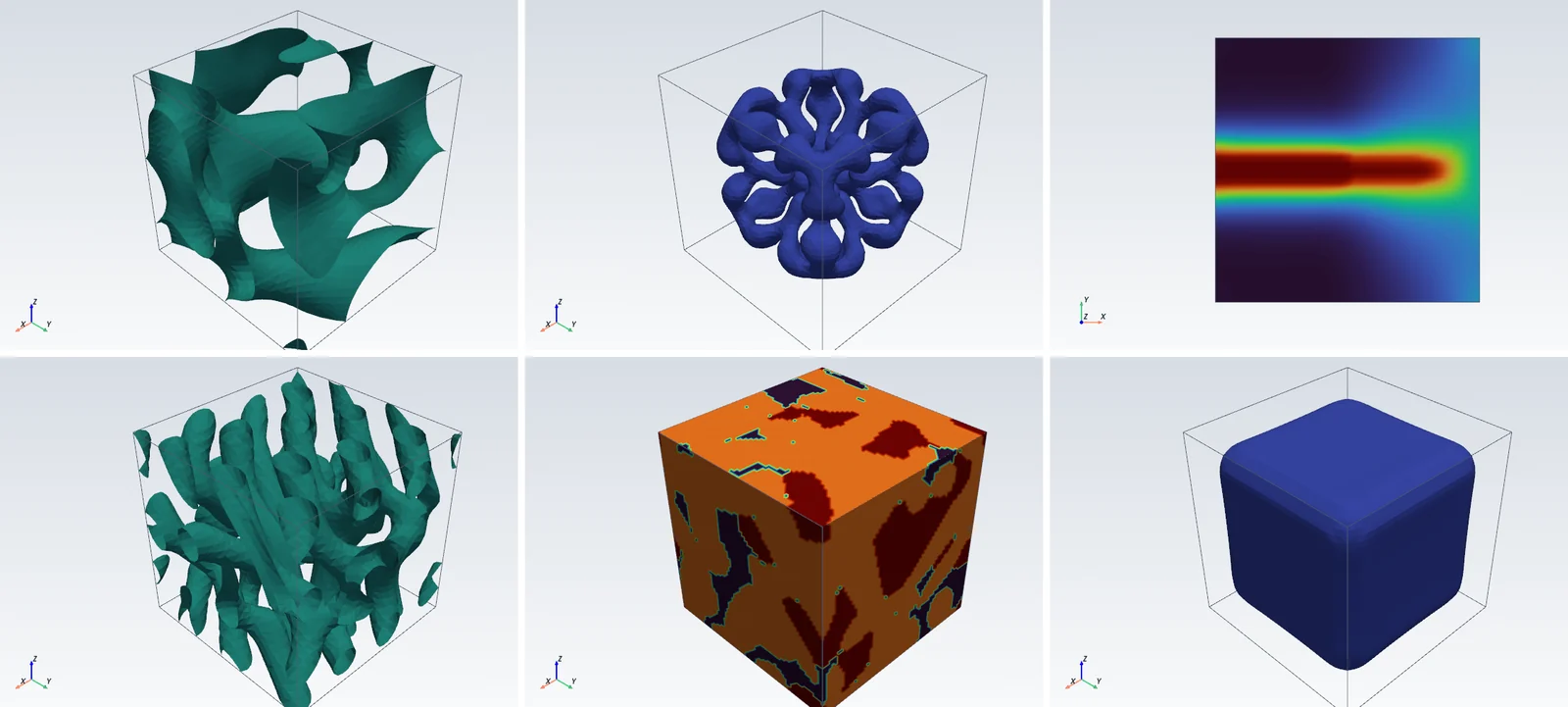 One engine, many physics. Spinodal decomposition, a Gray–Scott pattern, phase-field fracture, a phase-field crystal, glass-ceramic crystallization and solidification — each a short problem file shipped as an example.
Physics in the Examples
Each example is a complete problem file with its results, documented step by step.
Time Integration and Solvers
Explicit Runge–Kutta schemes, IMEX schemes that treat the stiff terms you mark implicitly, and fully implicit backward Euler and BDF2 for coupled and stationary equations. Error-controlled time steps reject and retry a step when its error or its Newton iteration fails, and land outputs at exact times; for quasi-static problems the same control becomes load stepping.
Newton's method uses the exact Jacobian, with an optional line search. Linear systems are equilibrated and solved by Krylov methods with Jacobi, incomplete-LU or algebraic multigrid preconditioning, or by a multithreaded direct solver where that is faster and fits in memory. A matrix that does not change is set up only once for the whole run. Long runs write checkpoints and continue from them; parameter sweeps run a study for a list of values and plot the results against them.
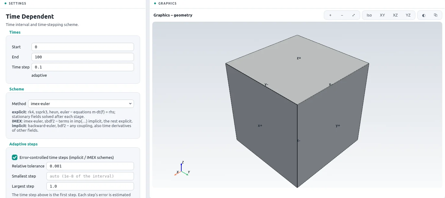 Study settings. Time scheme, error-controlled steps, output times and checkpoints.
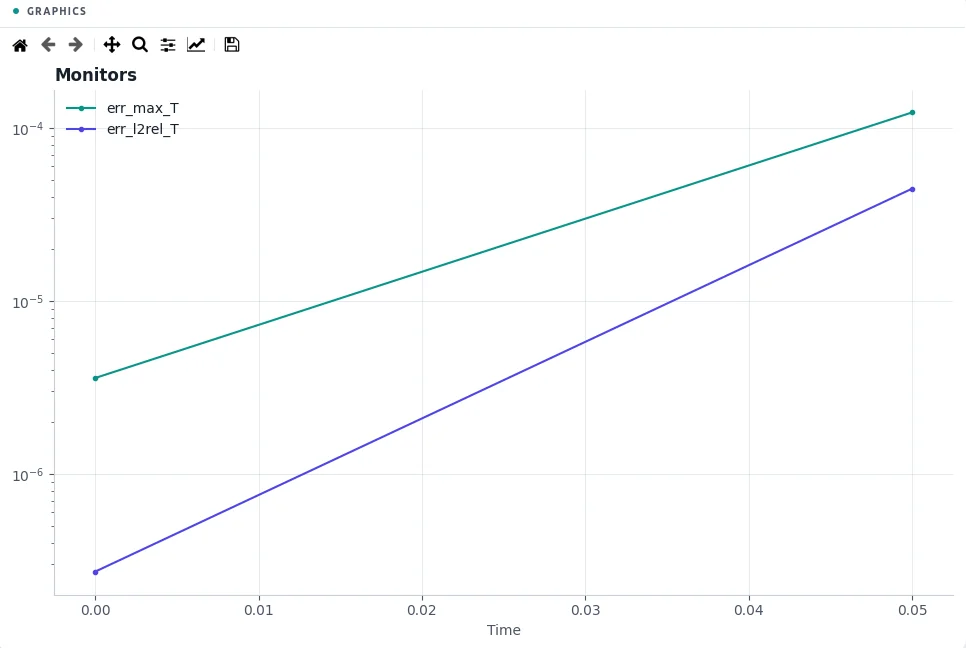 Verification mode. Give an exact solution and the engine adds the source terms and boundary data that make it the answer, then reports the error at every step.
Verified
- Second-order convergence at interior, face, edge and corner nodes, fourth derivatives included
- Every boundary-condition type checked with manufactured solutions, on boxes and curved parts
- Exact Jacobians agree with finite differences to about 10−10
- Cahn–Hilliard mass conserved to round-off on periodic domains
- Layered materials exact to round-off; composite sphere within 0.28 % of Lamé's solution
- Fibre composite within 0.5 % of Rayleigh's effective conductivity
- J2 plasticity and viscoelastic creep on their analytic curves
- Adaptive BDF2 second order; a restarted run identical to an uninterrupted one
Features
- Problems written as equations in a readable problem file; the interface edits the same file
- Model builder, settings and graphics laid out like common CAE tools, with light and dark themes
- Ready-made physics: heat transfer, solid mechanics, thermoelasticity, elastodynamics, diluted species, Cahn–Hilliard, Allen–Cahn, reaction–diffusion
- Syntax-highlighted expressions, completion of names, and undefined names underlined as you type
- Boxes, primitives, STEP and STL parts; boundary patches renamed, grouped and picked with the mouse
- Several materials with automatic interface conditions
- Local refinement by faces, boxes and spheres
- Dirichlet, Neumann, Robin and general equation conditions, per component and on parts of a face
- PDDO operators of order 2, 4 and 6, chosen from the equations
- Explicit, IMEX and implicit schemes with adaptive steps, checkpoints and restart
- Verification mode with manufactured solutions and error monitors
- 3D results as surfaces, slices, isosurfaces and points, on the deformed shape, animated over time
- Monitor plots, probe lines and points, parameter sweeps, all exportable as CSV
- ParaView output (VTK) of every stored time step
- Native C++/OpenMP kernels; Python hooks for model parts that are not PDEs
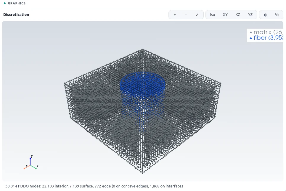 Several materials. The unit cell of a fibre composite, nodes coloured by region; the interface conditions come from the equations.
Who Is It For
- Research engineers whose model is not in a commercial package, or only behind a user subroutine
- Materials scientists simulating microstructure: phase separation, solidification, crystallization, precipitation
- Battery and electrochemistry teams coupling diffusion and mechanics
- Thermal and structural engineers working directly on CAD geometry
- Fracture and damage modelling with phase fields and history variables
- Teaching and research groups who want the equations, not the code, to be the model
Documentation
- User Manual — the interface, every part of the problem file, discretization, time stepping and solvers, results, and troubleshooting
- Examples — twenty documented problems, from verification cases to multigrain crystallization, each with its problem file and results
All Products