1The Problem
A battery electrode particle charged at constant current takes up lithium through its surface. The lithium swells the host lattice, and because the outer shell fills first it is compressed by the core, which pulls back on it. The hydrostatic stress in turn drives lithium towards regions of tension. Both couplings are solved together.
2The Problem File
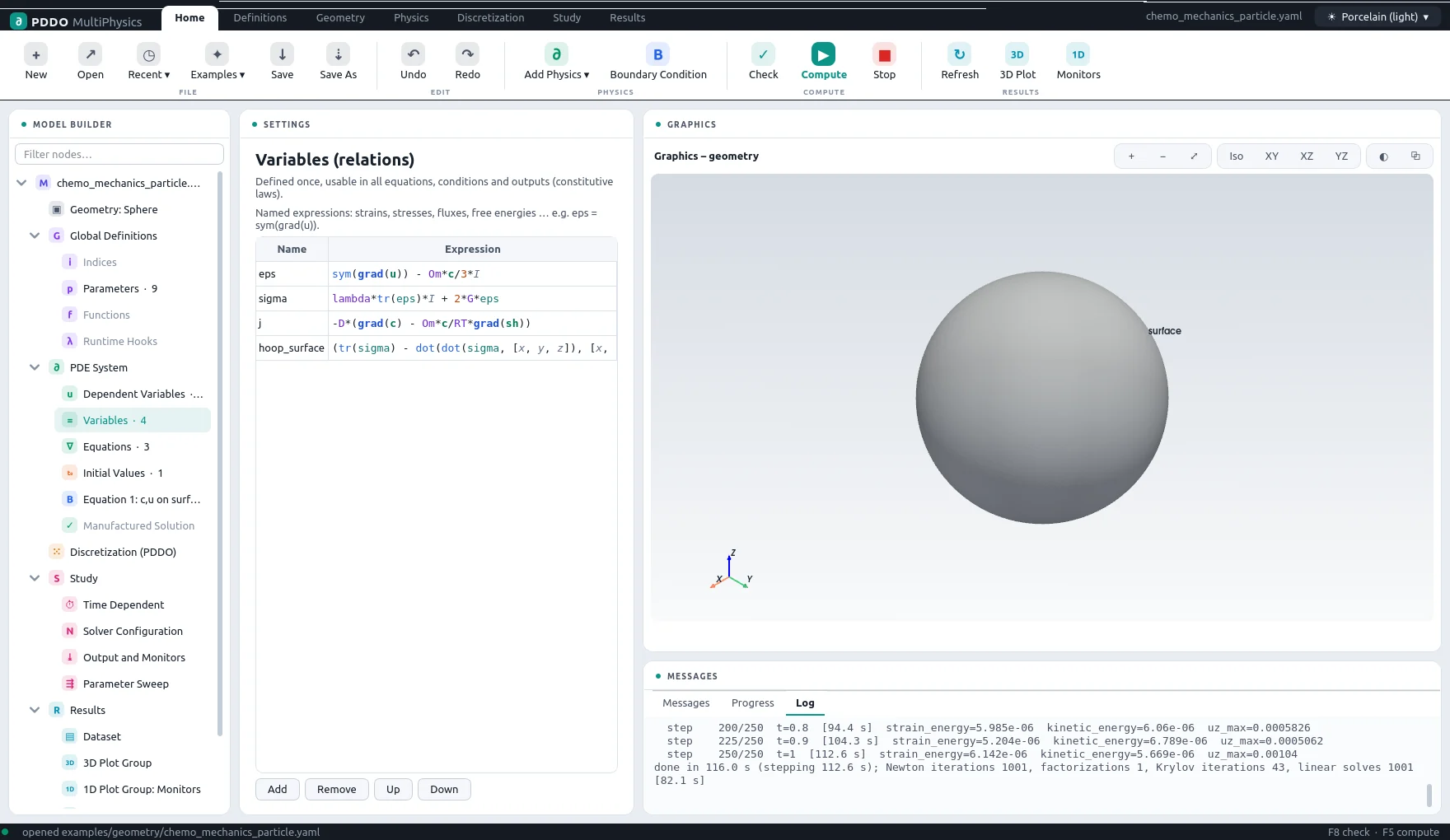
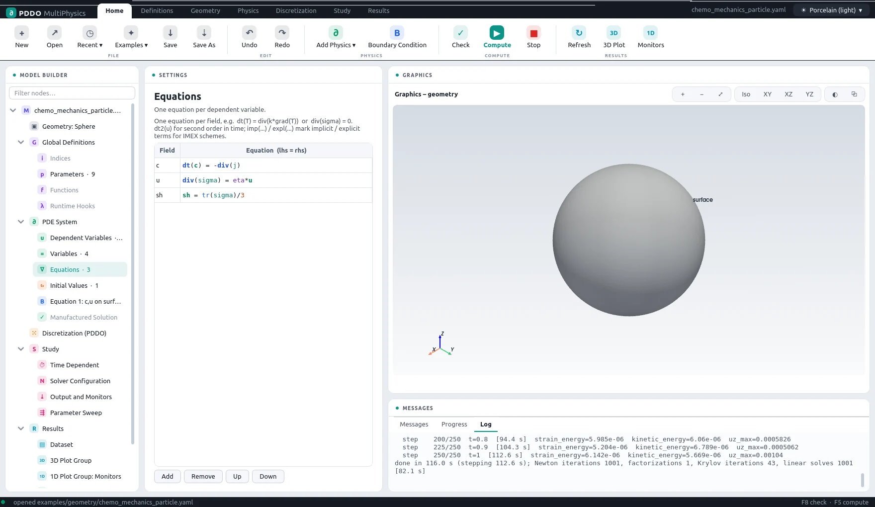
The hydrostatic stress is a field of its own, sh = tr(sigma)/3: its gradient
then needs only second derivatives of the displacement. The particle floats freely, so a tiny elastic
foundation removes the rigid-body modes. The coupling through c*grad(sh) is weakly
nonlinear, and newton: {reuse_jacobian: true} keeps one Jacobian and its solver for several steps.
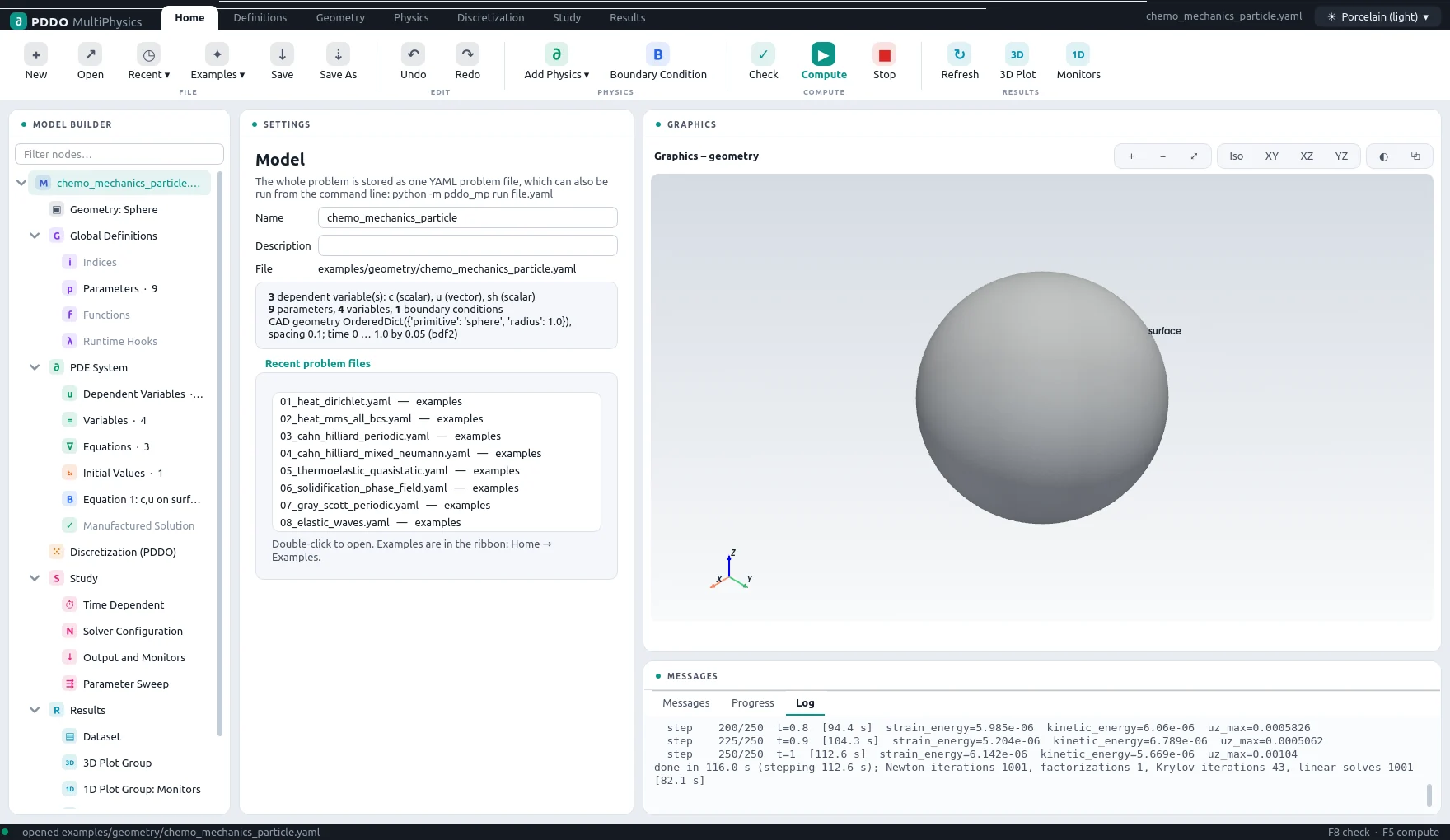
The complete problem file, examples/geometry/chemo_mechanics_particle.yaml
# Chemo-mechanics: lithium insertion into a spherical electrode particle (galvanostatic
# charging) with diffusion-induced stress and stress-assisted diffusion (two-way coupled):
#   dt(c) = -div(j),   j = -D (grad c - Om c/(R T) grad(sh)),   sh = tr(sigma)/3 (field)
#   div(sigma) = 0,    sigma = C : (eps - Om c/3 I)
# Surface: inward flux j0; traction free. The particle floats freely: a tiny elastic
# foundation (eta u) removes the rigid-body modes. Units: um, s, mol/um^3 scaled, GPa.
"k">name: chemo_mechanics_particle
"k">domain:
  "k">type: geometry
  "k">geometry: {primitive: sphere, radius: 1.0}
  "k">spacing: 0.1
"k">parameters:
  "k">E: 10.0
  "k">nu: 0.3
  "k">D: 1.0
  "k">Om: 0.05                     # partial molar volume (scaled)
  "k">RT: 2.5
  "k">j0: 0.1                      # insertion flux (inward)
  "k">eta: 1.0e-6
  "k">lambda: "E*nu/((1 + nu)*(1 - 2*nu))"
  "k">G: "E/(2*(1 + nu))"
"k">fields:
  "k">c: scalar
  "k">u: vector
  "k">sh: scalar                   # hydrostatic stress as a field: only 2nd derivatives (order 2)
"k">relations:
  "k">eps: "sym(grad(u)) - Om*c/3*I"
  "k">sigma: "lambda*tr(eps)*I + 2*G*eps"
  "k">j: "-D*(grad(c) - Om*c/RT*grad(sh))"
  "k">hoop_surface: "(tr(sigma) - dot(dot(sigma, [x, y, z]), [x, y, z])/(x**2 + y**2 + z**2))/2"
"k">equations:
  "k">c: "dt(c) = -div(j)"
  "k">u: "div(sigma) = eta*u"
  "k">sh: "sh = tr(sigma)/3"
"k">initial_conditions:
  "k">c: 0.0
"k">boundary_conditions:
  - "k">faces: [surface]
    "k">c: {equation: "dot(j, n) = -j0"}
    "k">u: {equation: "dot(sigma, n) = [0, 0, 0]"}
"k">time:
  "k">end: 1.0
  "k">dt: 0.05
  "k">scheme: bdf2
"k">solver:
  "k">newton: {reuse_jacobian: true}   # weak nonlinearity (c grad sh): reuse the factorization
"k">output:
  "k">every: 4
  "k">fields: [c, u, sh]
"k">monitors:
  "k">c_mean: "mean(c)"
  "k">c_max: "max(c)"
  "k">sigma_h_max: "max(sh)"
  "k">sigma_h_min: "min(sh)"
3Discretization
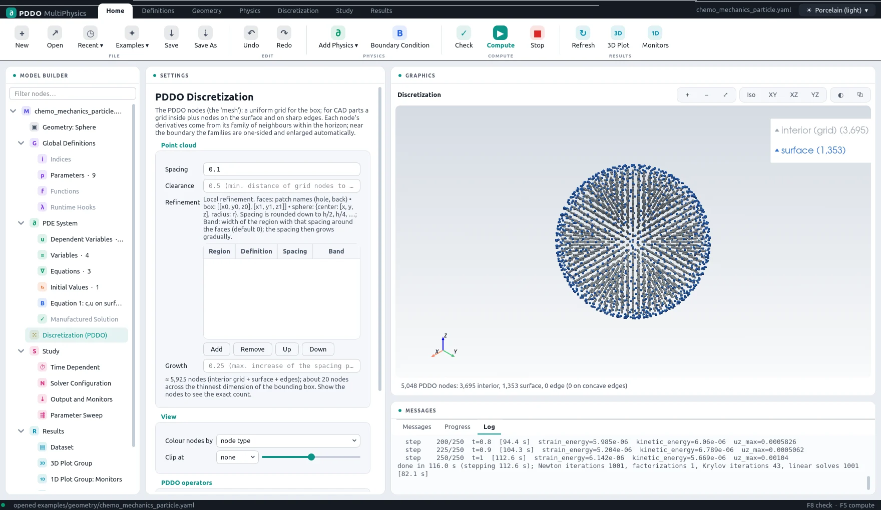
The sphere of radius 1 is filled at a spacing of 0.1 with 5,048 nodes.
4Results
- Nodes
- 5,048 (point cloud)
- PDDO order
- 2, horizon 2.015 Δx
- Time scheme
- bdf2
- Steps
- 20 × Δt = 0.05
- Newton iterations
- 28
- Factorizations
- 3
- Run time
- 4 min
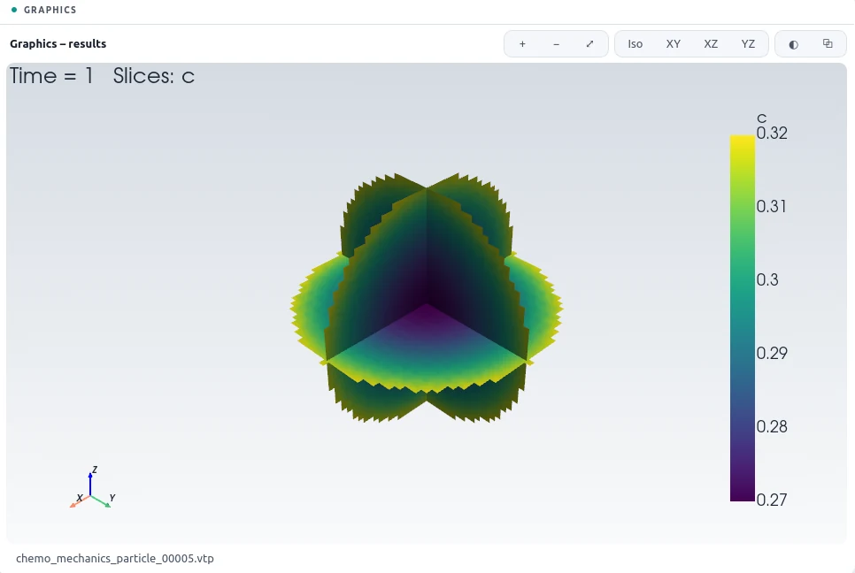
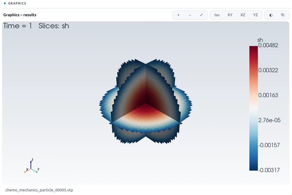
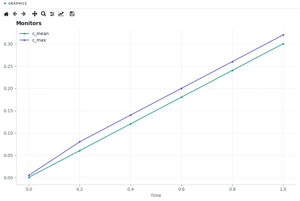
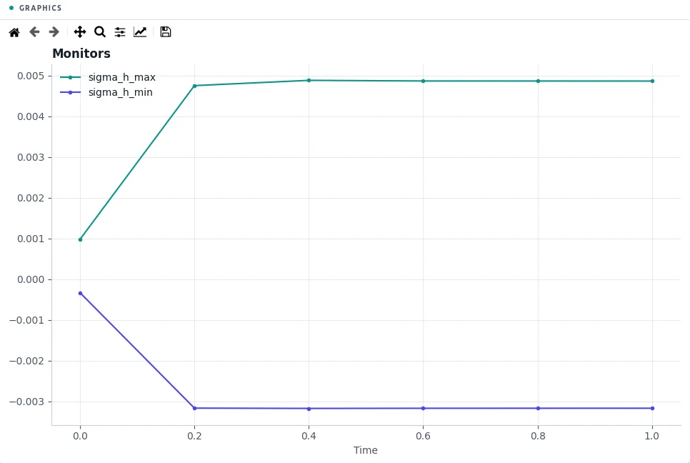
After t = 1 the mean concentration is 0.3003; the flux balance through the surface gives exactly 3j0t/R = 0.3000, a difference of 0.11 %. The highest concentration, 0.320, is at the surface. The hydrostatic stress ranges from -0.00317 (compression in the lithiated shell) to 0.00486 (tension in the core).
5Run It Yourself
The problem file ships with PDDO-MultiPhysics. Open it in the graphical interface and press Compute, or run it from the command line:
python -m pddo_mp gui examples/geometry/chemo_mechanics_particle.yaml
python -m pddo_mp run examples/geometry/chemo_mechanics_particle.yaml
Results go to results/chemo_mechanics_particle/
next to the problem file: a ParaView time series (.pvd), the monitors as CSV, and the
final state. Any entry can be changed on the command line, for example
--set time.end=0.5 for a run to half the end time. The user manual
describes every part of the problem file and of the interface.