1The Problem
In the Gray-Scott model, species v consumes species u autocatalytically while u is fed and v removed. With these feed and kill rates a small perturbation does not die out or fill the box uniformly; it splits and replicates into a pattern that spreads through the whole domain.
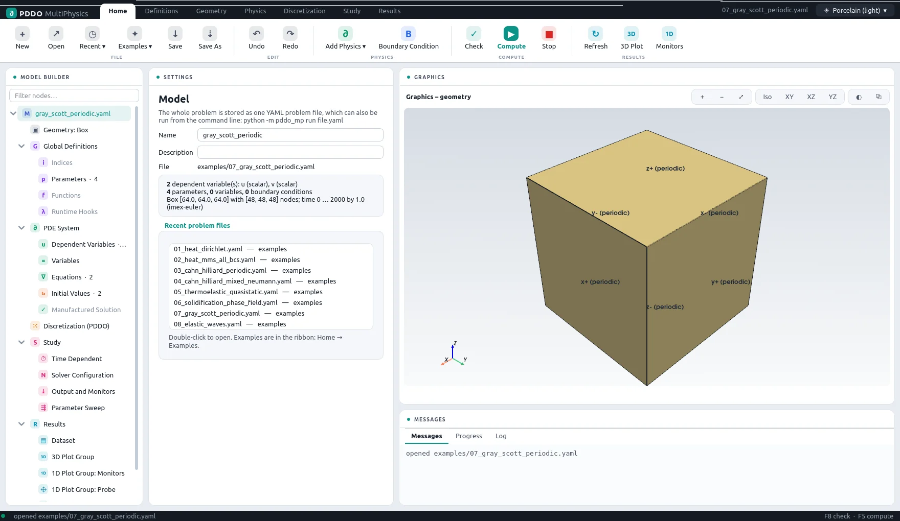
2The Problem File
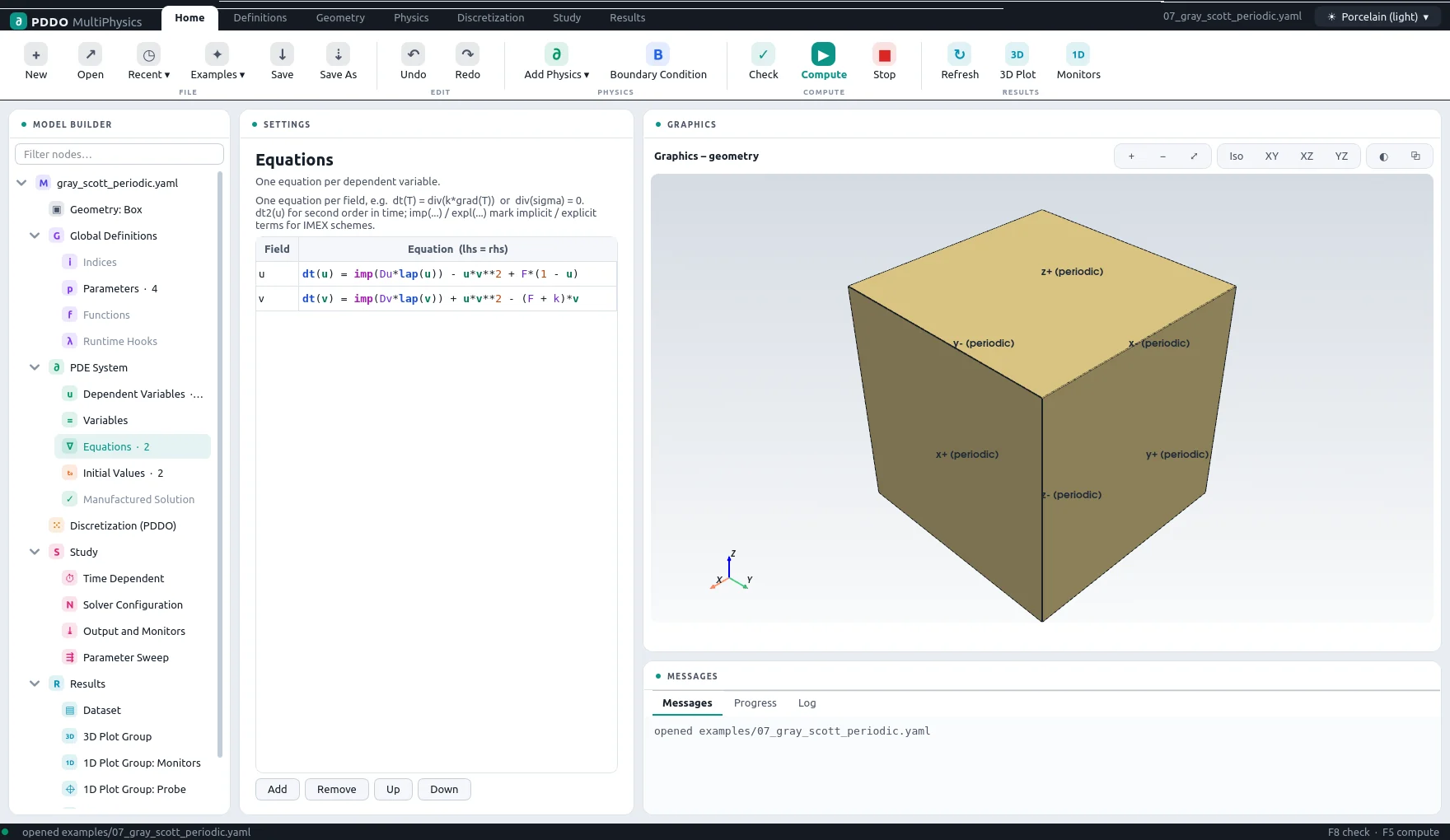
Two scalar fields and two equations, with diffusion marked imp() and the
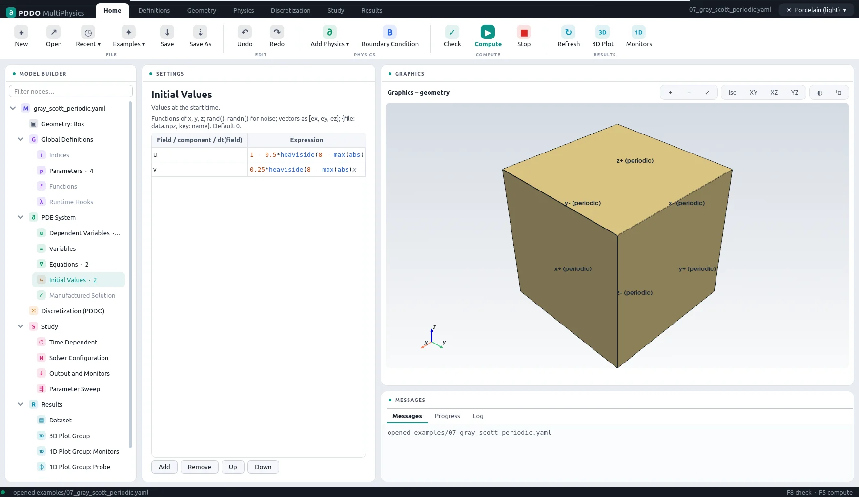
reactions explicit. The initial condition is a cube in the centre of the box, written with
heaviside and max(abs(...)), plus a little noise.
The complete problem file, examples/07_gray_scott_periodic.yaml
# Gray–Scott reaction–diffusion (pattern formation), periodic box.
#   dt(u) = Du lap(u) - u v^2 + F (1 - u)
#   dt(v) = Dv lap(v) + u v^2 - (F + k) v
# Diffusion implicit, reactions explicit (IMEX). A perturbed cube in the centre seeds the
# pattern.
"k">name: gray_scott_periodic
"k">domain:
  "k">size: [64, 64, 64]
  "k">n: [48, 48, 48]
  "k">periodic: [true, true, true]
"k">parameters:
  "k">Du: 0.16
  "k">Dv: 0.08
  "k">F: 0.035
  "k">k: 0.065
"k">fields:
  "k">u: scalar
  "k">v: scalar
"k">equations:
  "k">u: "dt(u) = imp(Du*lap(u)) - u*v**2 + F*(1 - u)"
  "k">v: "dt(v) = imp(Dv*lap(v)) + u*v**2 - (F + k)*v"
"k">initial_conditions:
  "k">u: "1 - 0.5*heaviside(8 - max(abs(x - 32), abs(y - 32), abs(z - 32))) + 0.02*(rand() - 0.5)"
  "k">v: "0.25*heaviside(8 - max(abs(x - 32), abs(y - 32), abs(z - 32))) + 0.02*(rand() - 0.5)"
"k">seed: 3
"k">time:
  "k">end: 2000
  "k">dt: 1.0
  "k">scheme: imex-euler
"k">output:
  "k">every: 100
"k">monitors:
  "k">v_mean: "mean(v)"
  "k">v_max: "max(v)"
3Results
- Nodes
- 48×48×48 = 110,592
- Periodic
- xyz
- PDDO order
- 2, horizon 2.015 Δx
- Time scheme
- imex-euler
- Steps
- 2,000 × Δt = 1
- Newton iterations
- 2,000
- Factorizations
- 0
- Run time
- 9 min
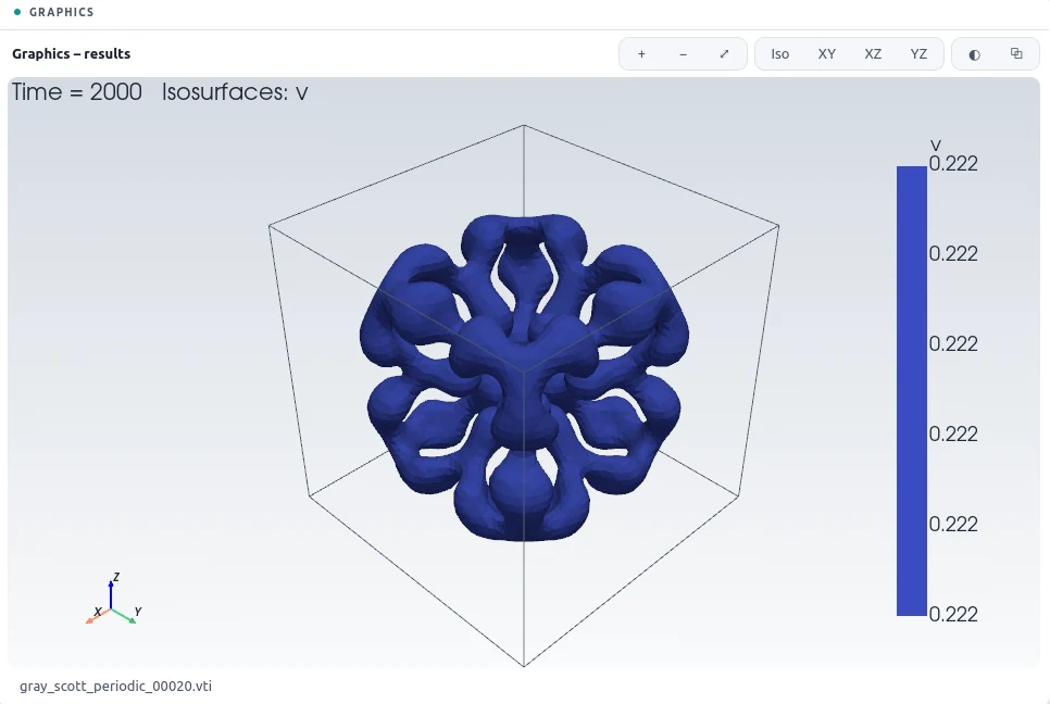
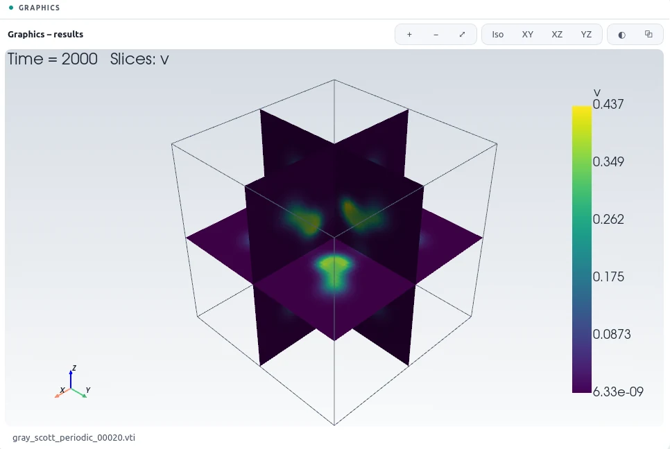
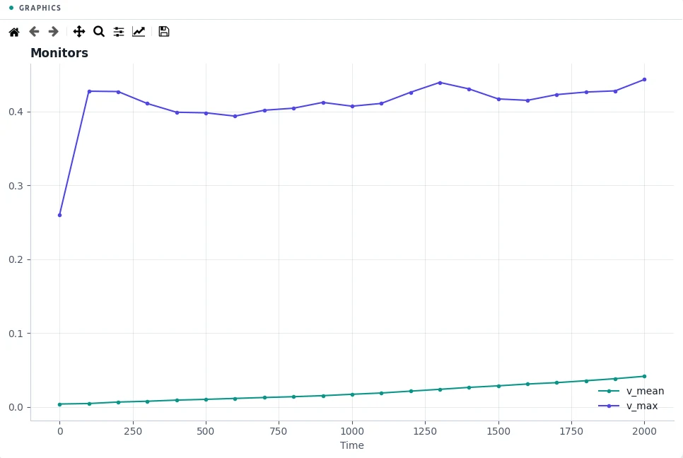
The seeded cube breaks up into lobes that split and replicate outward; by t = 2000 the pattern fills the middle of the box and is still spreading, so the mean of v keeps rising, from 0.0040 to 0.0415, while the largest value stays near 0.443.
4Run It Yourself
The problem file ships with PDDO-MultiPhysics. Open it in the graphical interface and press Compute, or run it from the command line:
python -m pddo_mp gui examples/07_gray_scott_periodic.yaml
python -m pddo_mp run examples/07_gray_scott_periodic.yaml
Results go to results/gray_scott_periodic/
next to the problem file: a ParaView time series (.pvd), the monitors as CSV, and the
final state. Any entry can be changed on the command line, for example
--set time.end=1000 for a run to half the end time. The user manual
describes every part of the problem file and of the interface.