Precipitation driven by a CALPHAD database | PDDO-MultiPhysics Examples

1The Problem

A crystal of the compound AB grows from an A-B liquid as the temperature ramps from 800 to 1000 K. How fast it grows depends on the thermodynamic driving force, which a CALPHAD database gives as a function of composition and temperature. The growing crystal takes up solute at its stoichiometric composition, depleting the surrounding liquid.

$$\frac{\partial\phi}{\partial t} = L\Big(\kappa\,\nabla^2\phi - W g'(\phi) + 6\,\Delta G(c, T)\,h'(\phi)\Big)$$

$$\frac{\partial c}{\partial t} = D\,\nabla^2 c - (x_p - c)\,\frac{\partial h(\phi)}{\partial t}$$

2The Problem File

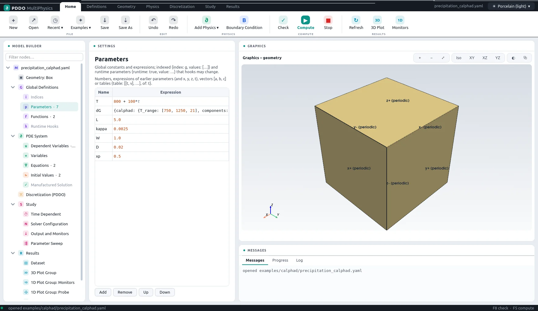
The driving force dG is a parameter defined by a calphad block: the database file ab_binary.tdb, the parent and product phases, and the composition and temperature ranges. The engine computes the parallel-tangent driving force with pycalphad once, tabulates it, caches the table, and interpolates it with cubic splines during the run. The temperature is itself a parameter, T: "800 + 100*t".

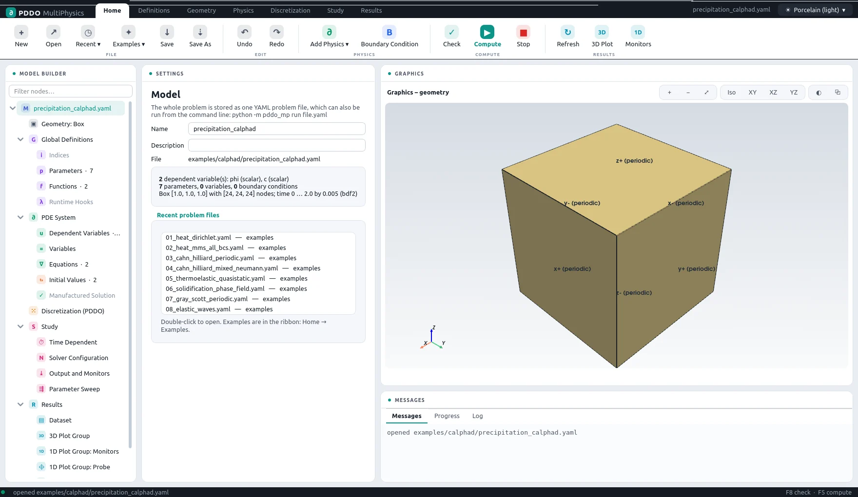
The complete problem file, examples/calphad/precipitation_calphad.yaml

# Growth of the stoichiometric compound AB from an A-B liquid during heating, driven by the
# CALPHAD driving force of the database ab_binary.tdb (parallel tangent, pycalphad):
#   dG_AB(x_B, T)  [J/mol / 1e4]  tabulated once over (x_B, T) and cached in .pddo_cache/
# Phase field phi (Allen-Cahn, double well + driving force), liquid composition c (diffusion,
# solute taken up by the growing AB crystal at x_B = 1/2).
"k">name: precipitation_calphad
"k">domain:
  "k">size: [1, 1, 1]
  "k">n: [24, 24, 24]
  "k">periodic: true
"k">parameters:
  "k">T: "800 + 100*t"                       # heating ramp (K)
  "k">dG:
    "k">calphad: {tdb: ab_binary.tdb, components: [A, B, VA], parent: LIQUID, phase: AB,
              "k">x: B, x_range: [0.02, 0.98, 49], T_range: [750, 1250, 21], scale: 1.0e4}
    "k">of: [c, T]
    "k">kind: cubic
  "k">L: 5.0
  "k">kappa: 2.5e-3               # interface width sqrt(kappa/W) = 0.05 (~1.6 nodes)
  "k">W: 1.0
  "k">D: 0.02
  "k">xp: 0.5
"k">functions:
  "k">h(p): "p**3*(10 - 15*p + 6*p**2)"
  "k">g(p): "p**2*(1 - p)**2"
"k">fields:
  "k">phi: scalar
  "k">c: scalar
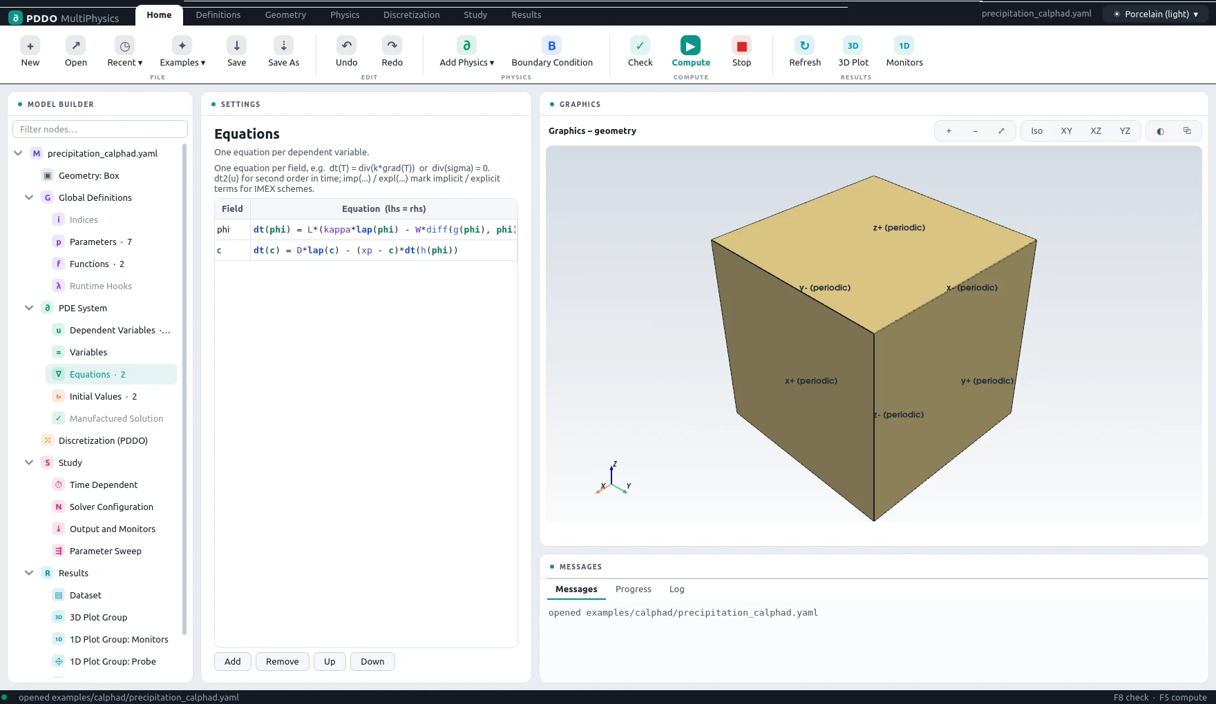
"k">equations:
  "k">phi: "dt(phi) = L*(kappa*lap(phi) - W*diff(g(phi), phi) + 6*dG*diff(h(phi), phi))"
  "k">c: "dt(c) = D*lap(c) - (xp - c)*dt(h(phi))"
"k">initial_conditions:
  "k">phi: "0.5*(1 - tanh((sqrt((x - 0.5)**2 + (y - 0.5)**2 + (z - 0.5)**2) - 0.2)/0.05))"
  "k">c: "0.42 + 0.005*randn()"
"k">time:
  "k">end: 2.0
  "k">dt: 0.005
  "k">scheme: bdf2
"k">output:
  "k">every: 20
"k">monitors:
  "k">solid_fraction: "mean(phi)"
  "k">c_mean: "mean(c)"
  "k">dG_max: "max(dG)"

**Figure 1.** The model in the GUI: the Model Builder tree on the left, the settings of the selected node in the middle, the graphics window on the right.

**Figure 2.** Parameters, including the CALPHAD driving force tabulated from the .tdb file and the heating ramp.

**Figure 3.** Phase field with the driving force, and solute diffusion with uptake by the growing crystal.

3Results

Nodes: 24×24×24 = 13,824
Periodic: xyz
PDDO order: 2, horizon 2.015 Δx
Time scheme: bdf2
Steps: 400 × Δt = 0.005
Newton iterations: 696
Factorizations: 0
Run time: 3 min

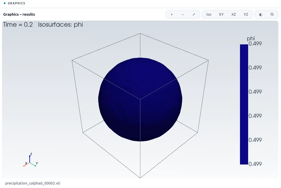
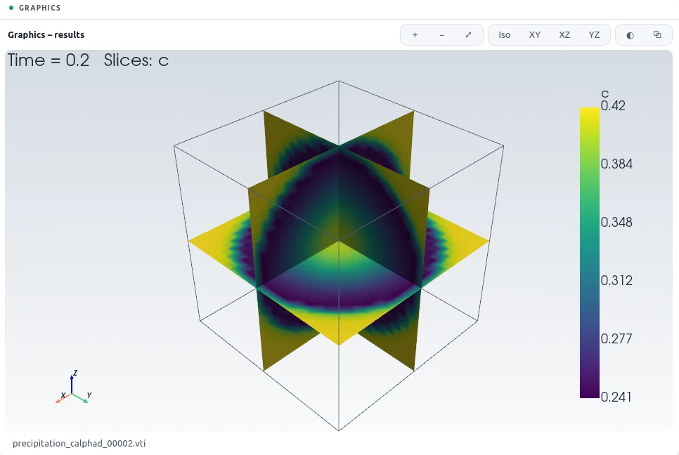
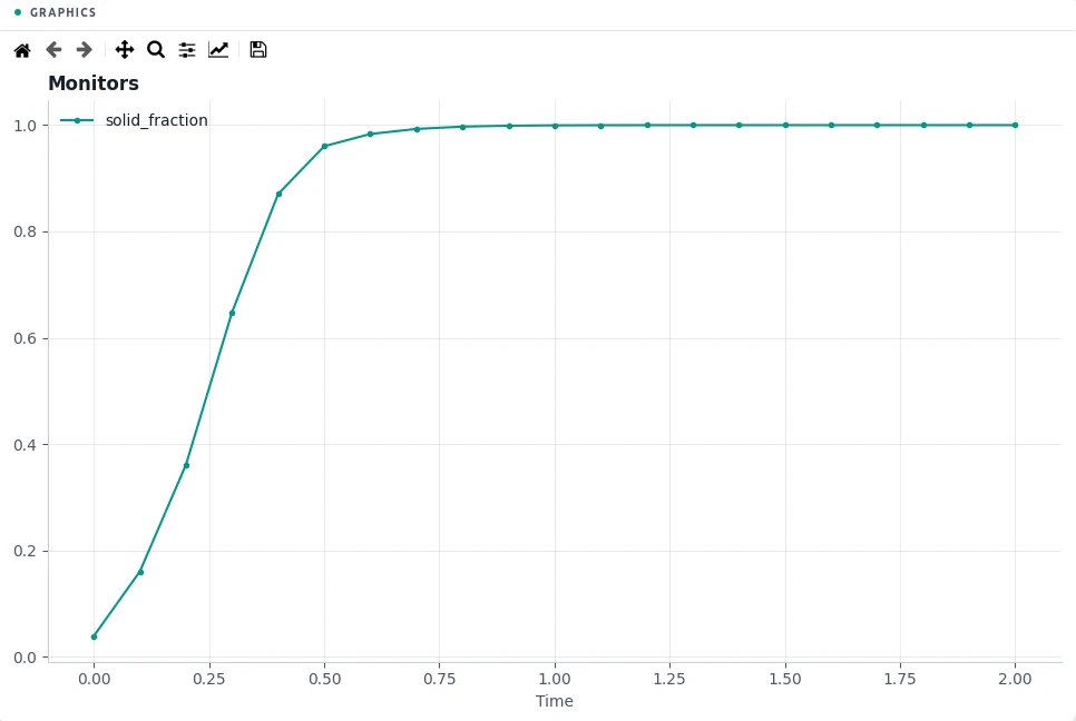
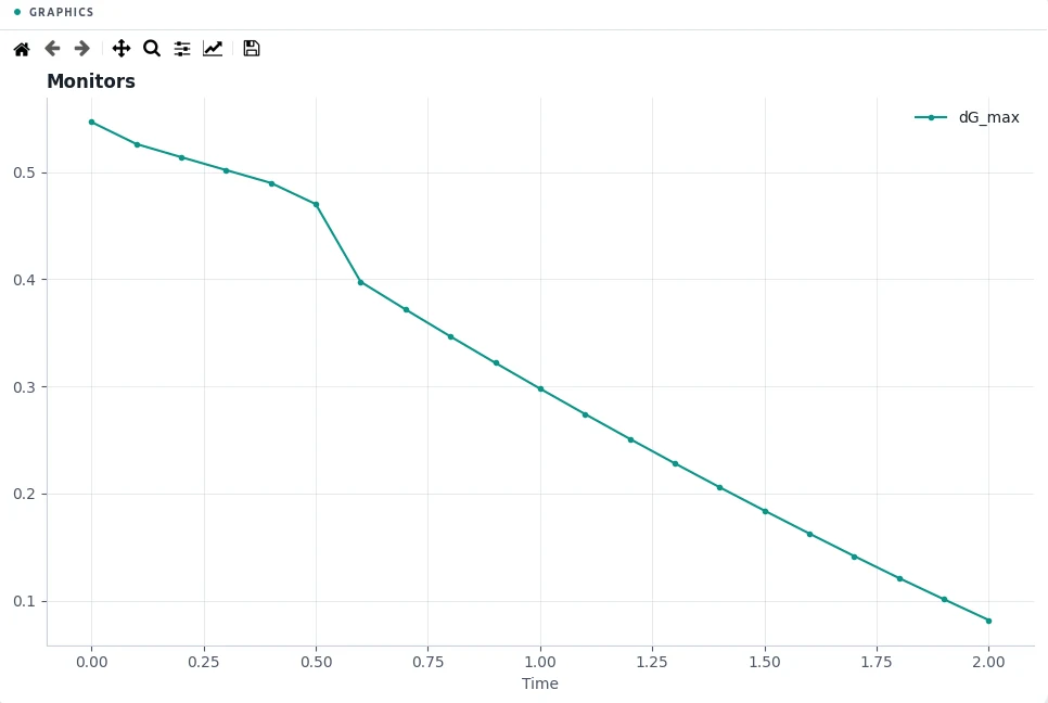
The seed, 3.9 % of the volume at the start, fills half the box by t = 0.25 and 95 % of it by t = 0.50: at these parameters the driving force stays positive as the liquid is depleted, so the compound eventually takes up the whole box. As it grows it takes up solute at x_B = 1/2, and the composition field falls from 0.420 to 0.213. The largest driving force falls from 0.547 to 0.0819 over the run.

**Figure 4.** The crystal (φ = 0.5) at t = 0.2, when it fills about a third of the box.

**Figure 5.** Composition on three slices at t = 0.2: the liquid depleted around the crystal.

**Figure 6.** Volume fraction of the crystal against time.

**Figure 7.** Largest driving force against time.

4Run It Yourself

The problem file ships with PDDO-MultiPhysics. Open it in the graphical interface and press Compute, or run it from the command line:

python -m pddo_mp gui examples/calphad/precipitation_calphad.yaml
python -m pddo_mp run examples/calphad/precipitation_calphad.yaml

Results go to results/precipitation_calphad/ next to the problem file: a ParaView time series (.pvd), the monitors as CSV, and the final state. Any entry can be changed on the command line, for example --set time.end=1 for a run to half the end time. The user manual describes every part of the problem file and of the interface.

1The Problem

2The Problem File

3Results

4Run It Yourself

Have a coupled problem of your own?