1The Problem
When the two phases of an alloy have different lattice parameters, phase separation builds up elastic energy. In a cubic crystal with Zener anisotropy 2.5 the <100> directions are soft, so the microstructure minimizes this energy by forming plates and rods along the cube axes instead of the random pattern of the purely chemical problem.
2The Problem File
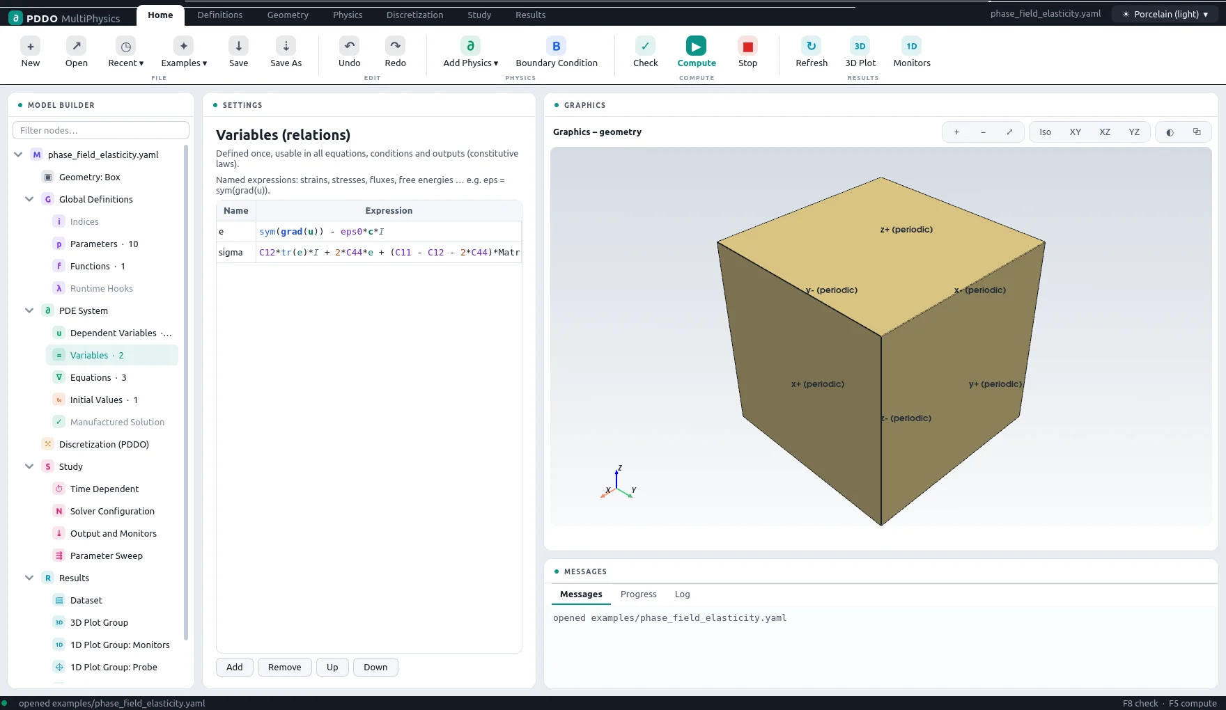
The cubic stiffness is written directly as an expression in the strain components,
C12*tr(e)*I + 2*C44*e + (C11 - C12 - 2*C44)*Matrix(...). The periodic body would be free
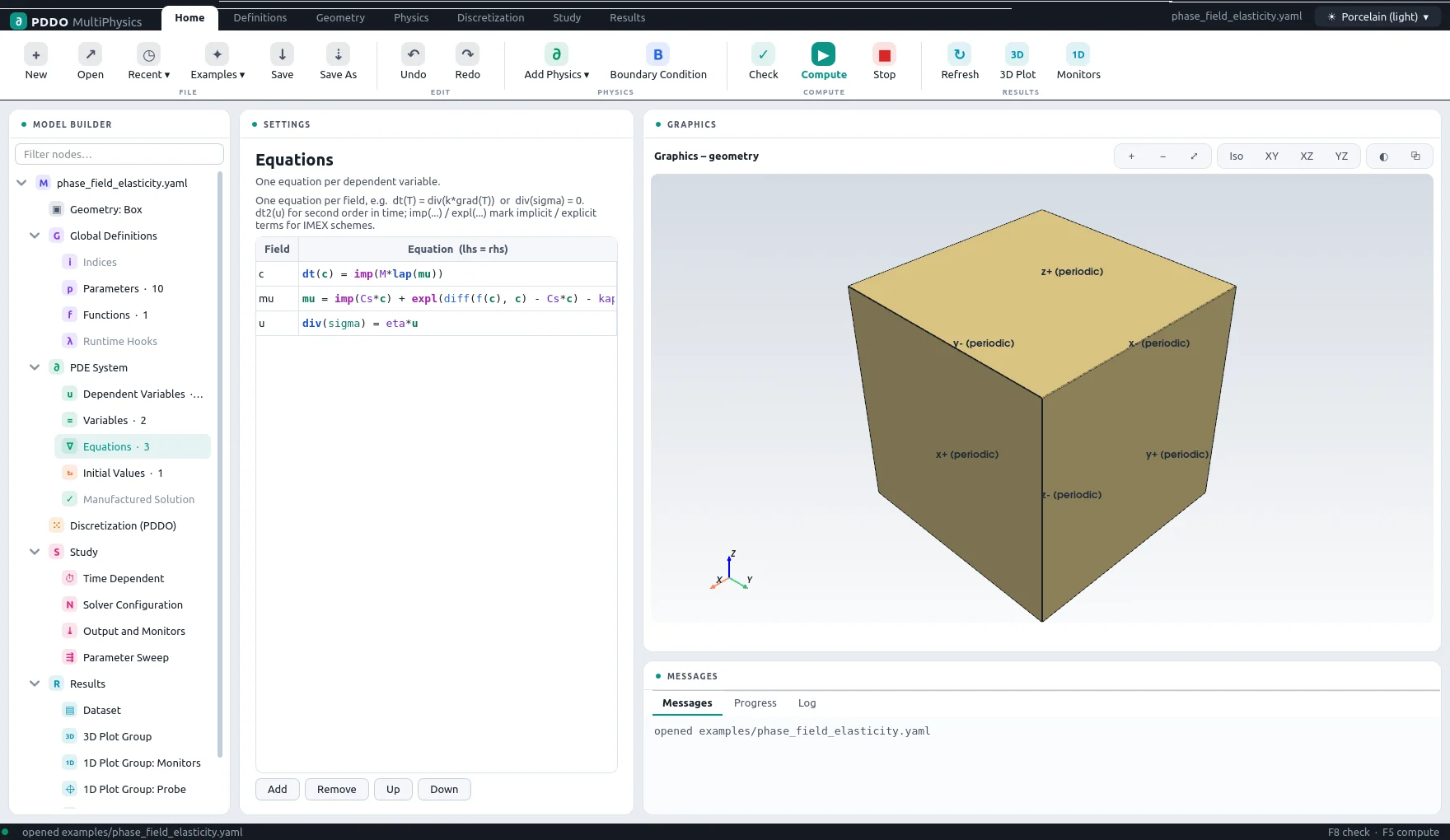
to translate, so a tiny elastic foundation, div(sigma) = eta*u, removes that rigid mode.
SBDF2 with a stabilized explicit f'(c) keeps the implicit matrix constant for the whole run.
The complete problem file, examples/phase_field_elasticity.yaml
# Phase field + elasticity: spinodal decomposition with a composition misfit in a cubic
# crystal (Cahn-Hilliard + small-strain elasticity, periodic):
#   dt(c) = M lap(mu),   mu = f'(c) - kappa lap(c) - eps0 tr(sigma)
#   div(sigma) = 0,      sigma = C_cubic : (eps - eps0 c I)
# Cubic elasticity with Zener anisotropy 2 C44/(C11 - C12) = 2.5: the <100> directions are
# elastically soft, so the two phases form plates / rods aligned with the cube axes.
# IMEX (SBDF2): f'(c) explicit with a linear stabilization; everything else implicit and
# linear, so one factorization serves the whole run. A tiny elastic foundation (eta u)
# fixes the rigid translation of the periodic body.
"k">name: phase_field_elasticity
"k">domain:
  "k">size: [24, 24, 24]
  "k">n: [24, 24, 24]                  # dx = 1; 32^3 needs ~2 x 20 GB to factorize
  "k">periodic: true
"k">parameters:
  "k">M: 1.0
  "k">kappa: 1.0
  "k">W: 1.0
  "k">Cs: 2.0                          # stabilization of the explicit f'(c)
  "k">C11: 250.0
  "k">C12: 150.0
  "k">C44: 125.0
  "k">eps0: 0.03                       # misfit strain per unit composition
  "k">eta: 1.0e-6
  "k">c0: 0.5
"k">functions:
  "k">f(c): "W*c**2*(1 - c)**2"
"k">fields:
  "k">c: scalar
  "k">mu: scalar
  "k">u: vector
"k">relations:
  "k">e: "sym(grad(u)) - eps0*c*I"
  "k">sigma: >-
    C12*tr(e)*I + 2*C44*e + (C11 - C12 - 2*C44)*Matrix([[e[0, 0], 0, 0],
    [0, e[1, 1], 0], [0, 0, e[2, 2]]])
"k">equations:
  "k">c: "dt(c) = imp(M*lap(mu))"
  "k">mu: "mu = imp(Cs*c) + expl(diff(f(c), c) - Cs*c) - kappa*lap(c) - eps0*tr(sigma)"
  "k">u: "div(sigma) = eta*u"
"k">initial_conditions:
  "k">c: "c0 + 0.02*randn()"
"k">time:
  "k">end: 300.0
  "k">dt: 1.0
  "k">scheme: sbdf2
"k">output:
  "k">every: 50
  "k">fields: [c, u]
"k">monitors:
  "k">c_mean: "mean(c)"
  "k">c_min: "min(c)"
  "k">c_max: "max(c)"

3Results
- Nodes
- 24×24×24 = 13,824
- Periodic
- xyz
- PDDO order
- 2, horizon 2.015 Δx
- Time scheme
- sbdf2
- Steps
- 300 × Δt = 1
- Newton iterations
- 301
- Factorizations
- 2
- Run time
- 18 min
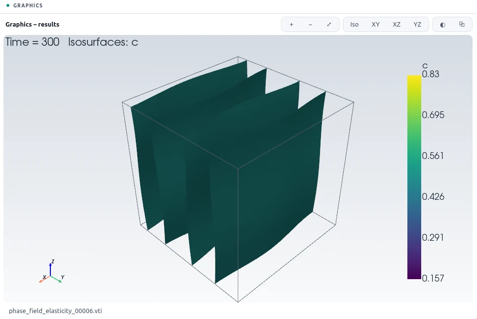
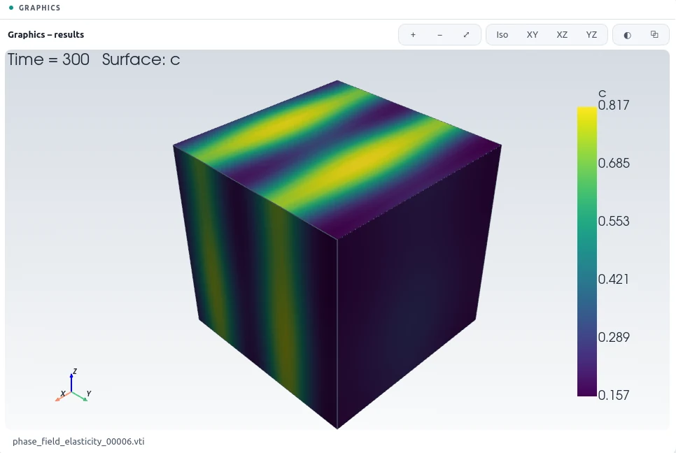
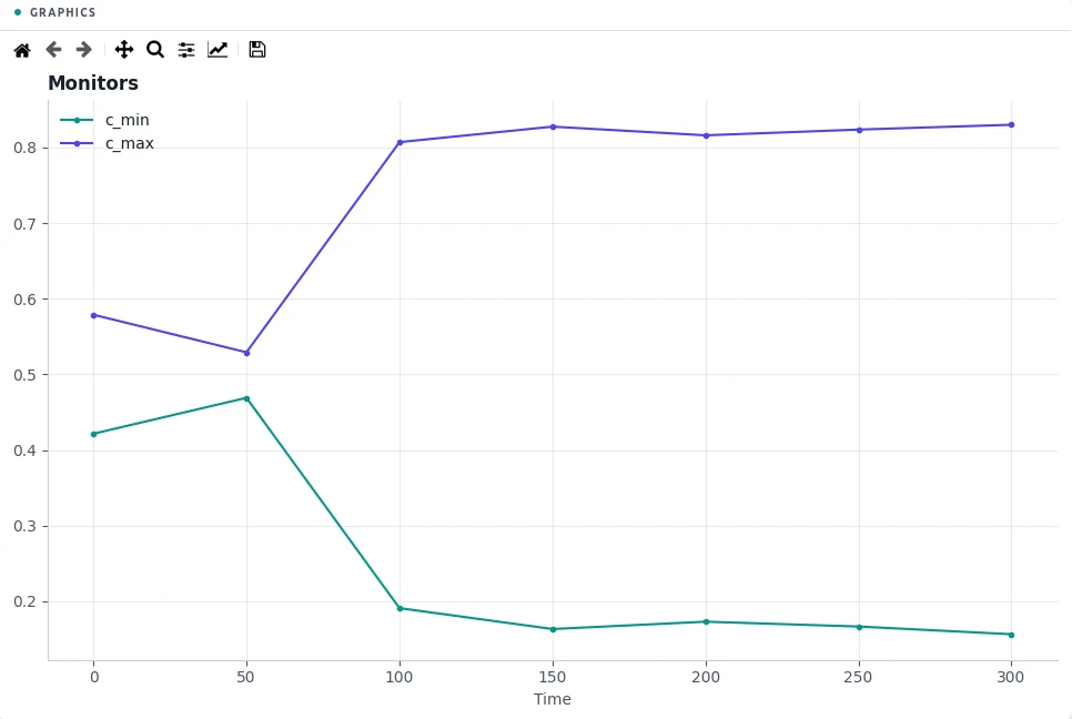
By t = 300 the composition has separated into phases between 0.157 and 0.830, arranged as parallel plates normal to one cube axis, the elastically soft direction, instead of the interconnected pattern of the purely chemical problem. The mean composition changes by less than 1×10⁻¹⁰. Jacobi-GMRES stalls on this coupled system, so the solver factorizes the constant implicit matrix instead (2 factorizations in the whole run); after that each step takes about a second.
4Run It Yourself
The problem file ships with PDDO-MultiPhysics. Open it in the graphical interface and press Compute, or run it from the command line:
python -m pddo_mp gui examples/phase_field_elasticity.yaml
python -m pddo_mp run examples/phase_field_elasticity.yaml
Results go to results/phase_field_elasticity/
next to the problem file: a ParaView time series (.pvd), the monitors as CSV, and the
final state. Any entry can be changed on the command line, for example
--set time.end=150 for a run to half the end time. The user manual
describes every part of the problem file and of the interface.