Heat conduction against the exact solution | PDDO-MultiPhysics Examples

1The Problem

A unit cube starts from a single sine mode of temperature and cools through its faces, which are held at T = 0. The mode keeps its shape and decays exponentially, so the exact solution is known at every point and every time.

$$\frac{\partial T}{\partial t} = a\,\nabla^2 T \quad\text{in } (0,1)^3, \qquad T = 0 \text{ on all faces}$$

$$T(\mathbf{x},t) = e^{-3\pi^2 a t}\,\sin \pi x\,\sin \pi y\,\sin \pi z$$

2The Problem File

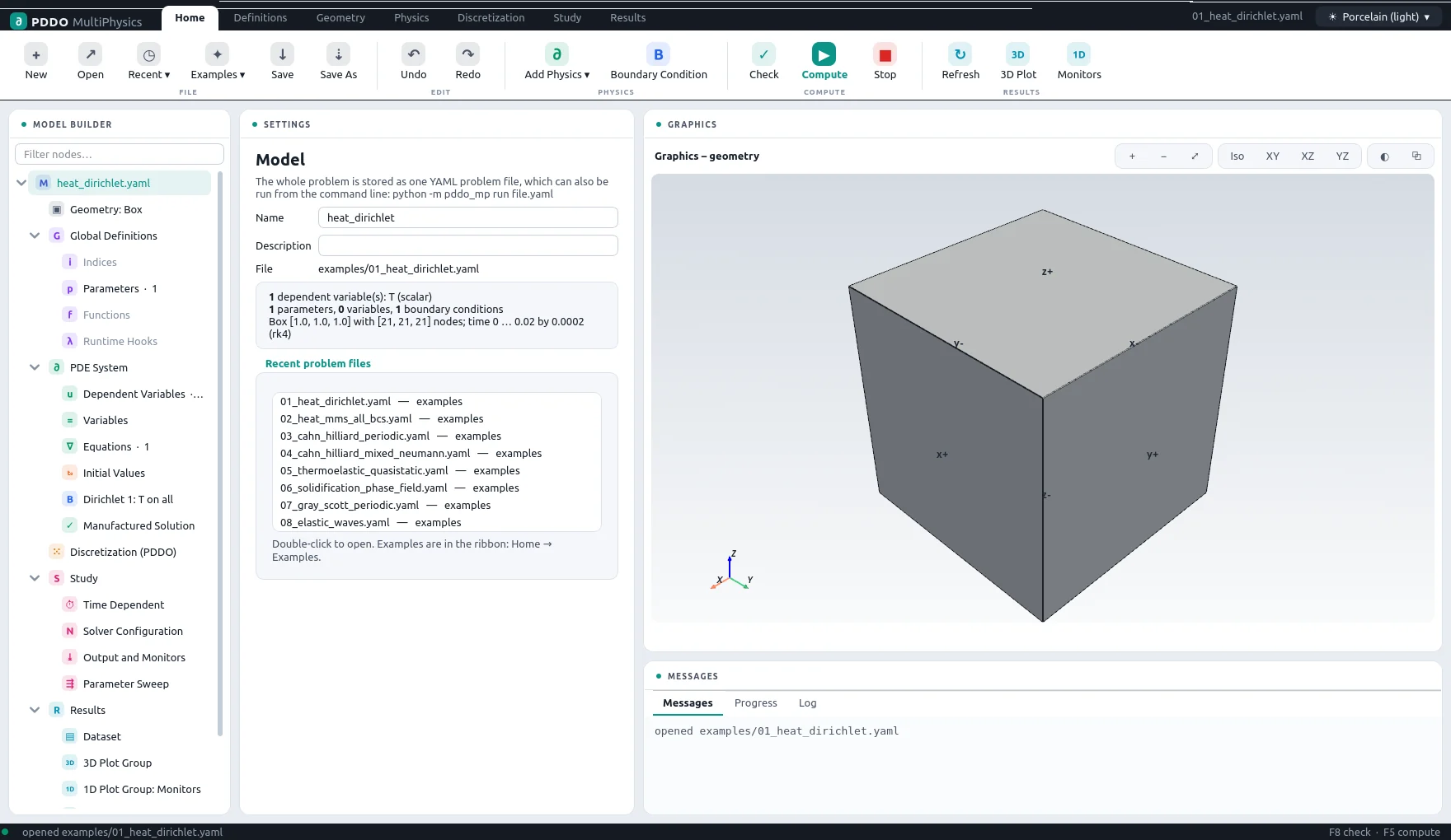
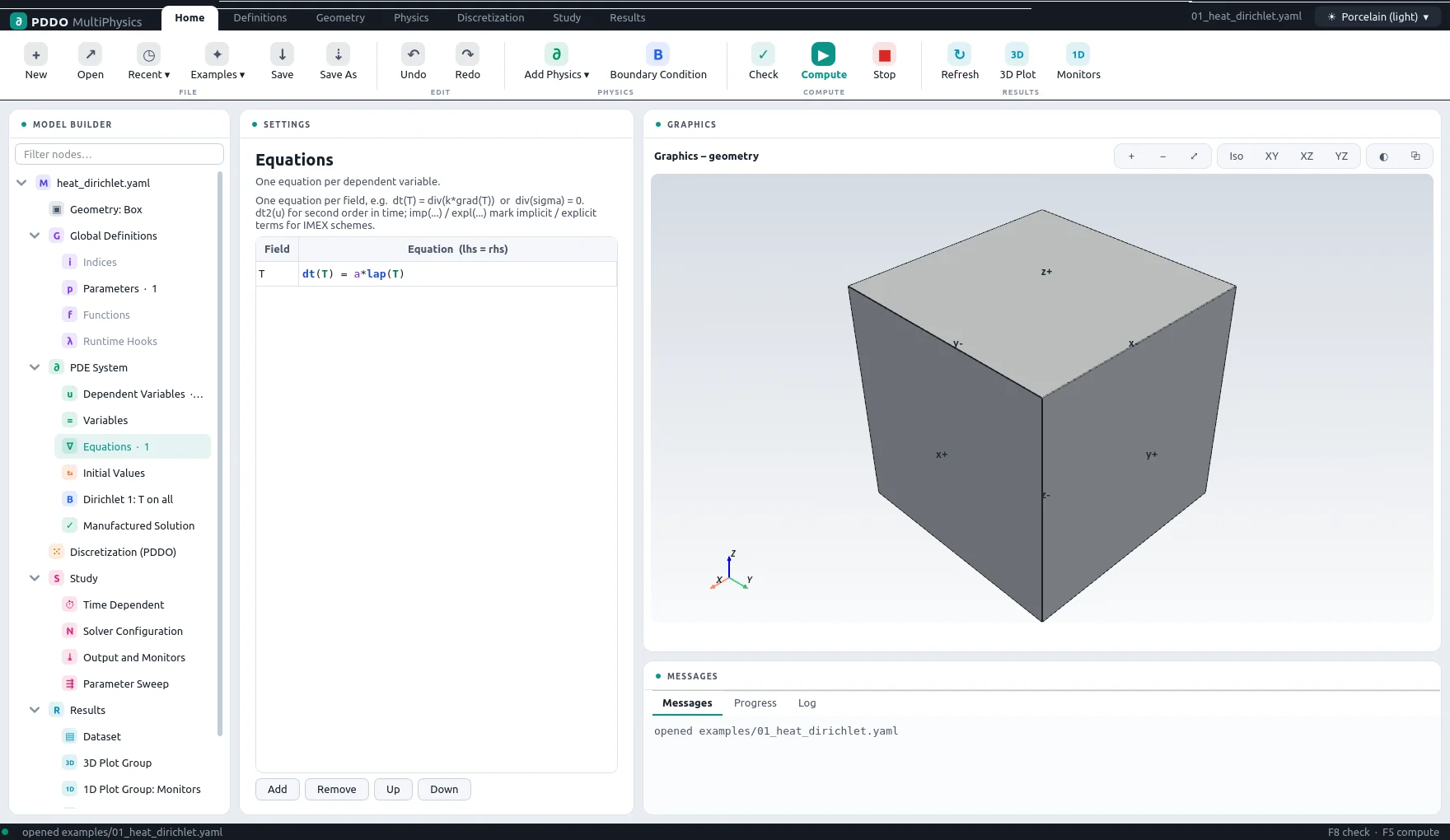
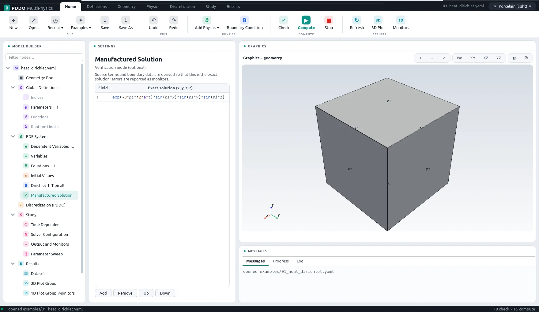
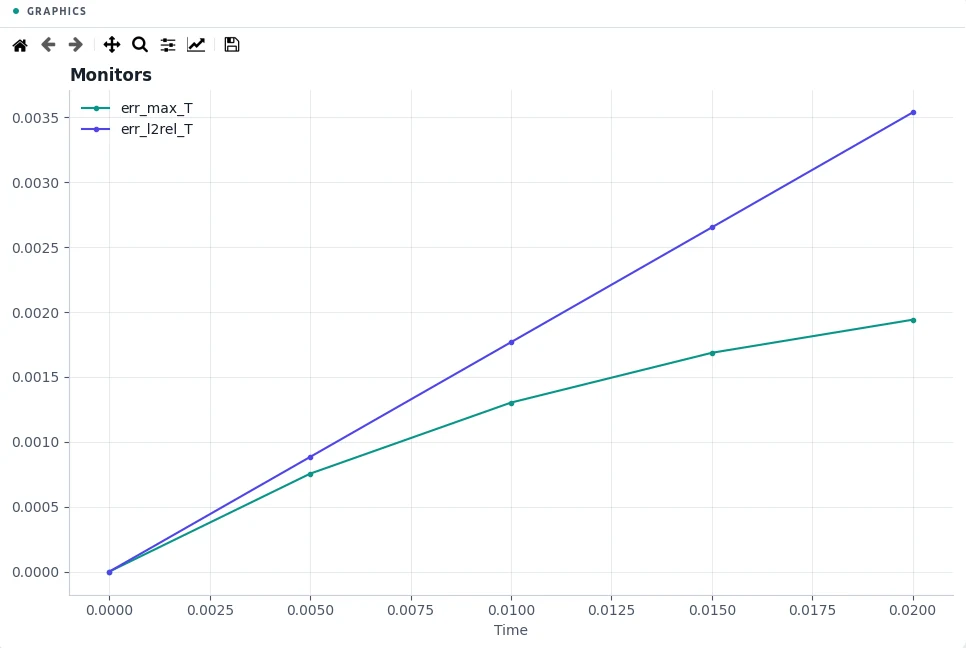
The whole model is one equation, dt(T) = a*lap(T), one boundary condition on all faces, and the exact solution under manufactured. A manufactured solution does three things: it sets the initial condition, it adds the source term it would need (zero here, since it already satisfies the equation), and it adds the monitors err_max_T and err_l2rel_T, the largest and the relative L2 error at every output step. The time scheme is the explicit fourth-order Runge-Kutta method; replace rk4 with bdf2, crank-nicolson or any other scheme to compare them on the same problem.

The complete problem file, examples/01_heat_dirichlet.yaml

# Transient heat conduction in a unit cube, T = 0 on all faces.
# The exact solution T = exp(-3 pi^2 a t) sin(pi x) sin(pi y) sin(pi z) is given as a
# "manufactured" solution: it sets the initial condition and adds error monitors
# (the source term it would add is zero here).
"k">name: heat_dirichlet
"k">domain:
  "k">type: box
  "k">size: [1, 1, 1]
  "k">n: [21, 21, 21]
"k">parameters:
  "k">a: 1.0                       # diffusivity
"k">fields:
  "k">T: scalar
"k">equations:
  "k">T: "dt(T) = a*lap(T)"
"k">boundary_conditions:
  - "k">faces: all
    "k">T: {dirichlet: 0}
"k">manufactured:
  "k">T: "exp(-3*pi**2*a*t)*sin(pi*x)*sin(pi*y)*sin(pi*z)"
"k">time:
  "k">end: 0.02
  "k">dt: 2.0e-4
  "k">scheme: rk4
"k">output:
  "k">every: 25
"k">monitors:
  "k">T_max: "max(T)"
  "k">heat: "integral(T)"

**Figure 1.** The model in the GUI: the Model Builder tree on the left, the settings of the selected node in the middle, the graphics window on the right.

**Figure 2.** The equation as typed in the Equations node. Operators, fields and parameters are highlighted; an undefined name would be underlined.

**Figure 3.** The Manufactured Solution node holds the exact solution. It provides the initial condition and the error monitors.

3Results

Nodes: 21×21×21 = 9,261
PDDO order: 2, horizon 2.015 Δx
Time scheme: rk4
Steps: 100 × Δt = 0.0002
Newton iterations: 0
Factorizations: 0
Run time: 1 s

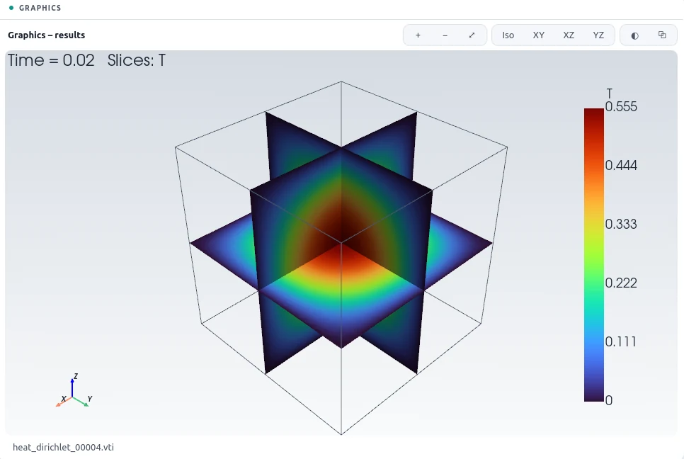
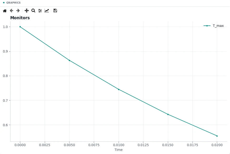
At t = 0.020 the largest temperature is 0.5551; the exact value is 0.5531. The relative L2 error over the cube is 0.35 % and the largest pointwise error 0.0019. Repeating the run on finer grids shows the second-order convergence of the spatial operators (the verification suite does this for every scheme).

**Figure 4.** Temperature on three slices through the cube at the final time.

**Figure 5.** The error monitors against time: the largest and the relative L2 error of T.

**Figure 6.** The largest temperature decaying as exp(−3π²at).

4Run It Yourself

The problem file ships with PDDO-MultiPhysics. Open it in the graphical interface and press Compute, or run it from the command line:

python -m pddo_mp gui examples/01_heat_dirichlet.yaml
python -m pddo_mp run examples/01_heat_dirichlet.yaml

Results go to results/heat_dirichlet/ next to the problem file: a ParaView time series (.pvd), the monitors as CSV, and the final state. Any entry can be changed on the command line, for example --set time.end=0.01 for a run to half the end time. The user manual describes every part of the problem file and of the interface.

1The Problem

2The Problem File

3Results

4Run It Yourself

Have a coupled problem of your own?