Nonlinear heat conduction with every boundary condition | PDDO-MultiPhysics Examples

1The Problem

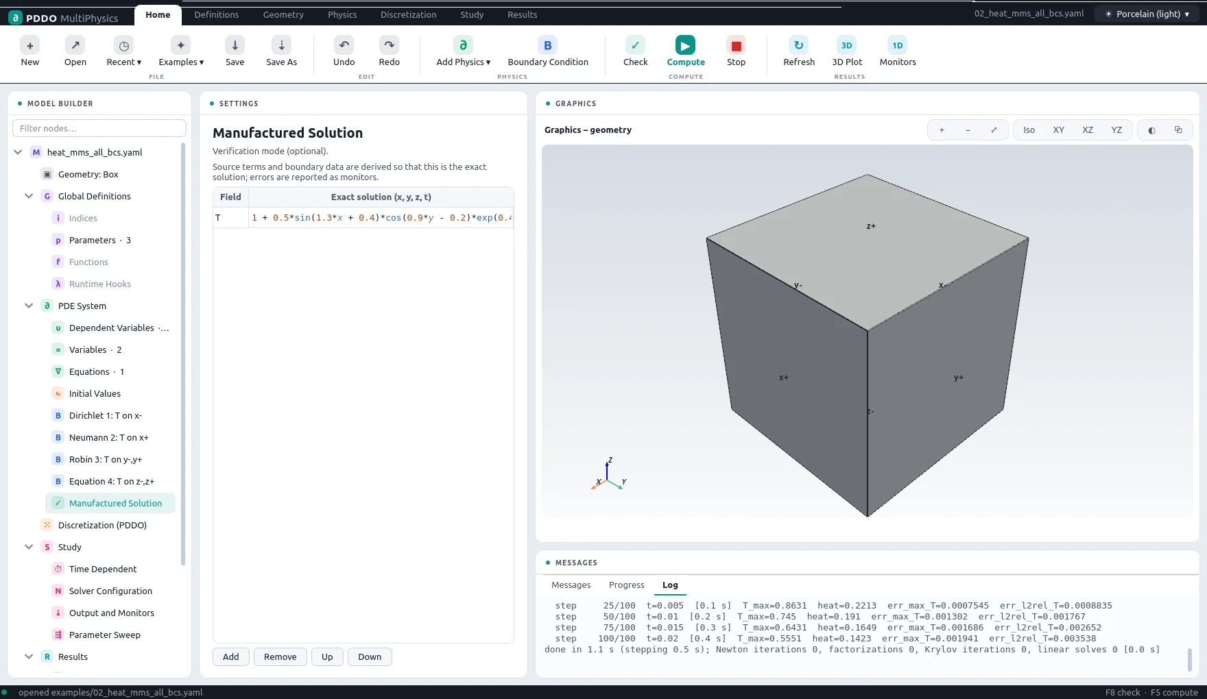
The conductivity grows with the square of the temperature, which makes the problem nonlinear, and each pair of faces carries a different kind of condition: a time-dependent Dirichlet value, a Neumann condition, a Robin condition, and a general flux equation for convection. Instead of an exact solution of this problem, which does not exist in closed form, a smooth function is chosen and the engine derives the source term and all the boundary data that make it the solution. The difference between the computed and the chosen field is then the discretization error alone.

$$\frac{\partial T}{\partial t} = -\nabla\cdot\mathbf{q} + s, \qquad \mathbf{q} = -k(T)\,\nabla T, \qquad k(T) = k_0\,(1 + \beta T^2)$$

$$T_{\text{exact}} = 1 + \tfrac12 \sin(1.3x + 0.4)\,\cos(0.9y - 0.2)\,e^{0.4z}\,e^{-t}$$

2The Problem File

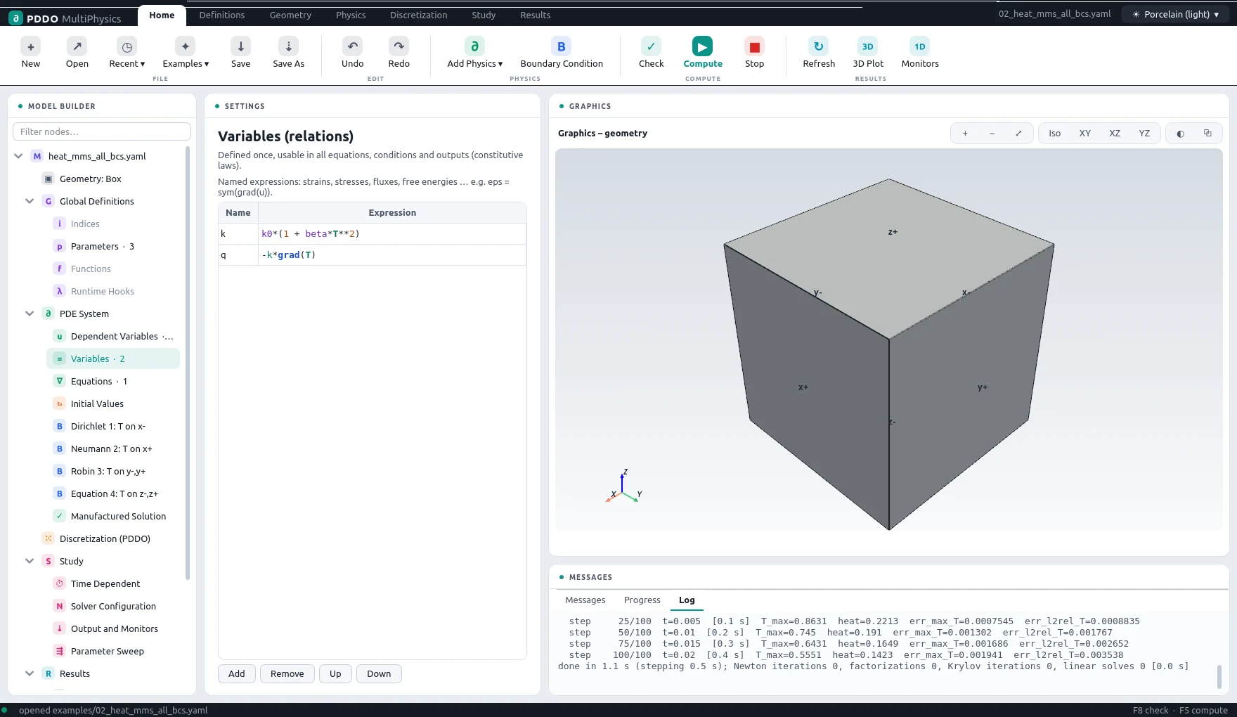
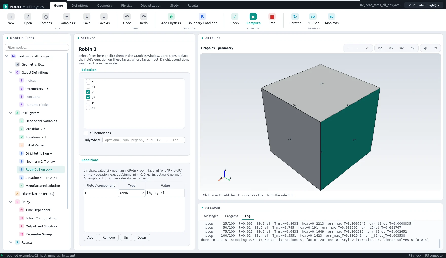
The flux is written once as a relation, q = -k*grad(T), with k = k0*(1 + beta*T**2), and the equation uses it as dt(T) = -div(q). The engine differentiates the nonlinear flux symbolically, both for the PDDO derivatives and for the exact Jacobian of the Newton solver. The four boundary conditions show the four forms:

Faces	Condition	Meaning
x−	`{dirichlet: 0}`	value prescribed (replaced by the exact data in manufactured mode)
x+	`{neumann: 0}`	normal derivative prescribed
y−, y+	`{robin: [h, 1, 0]}`	h·T + dT/dn = g
z−, z+	`{equation: "dot(q, n) = h*T"}`	any equation in the fields, relations and the outward normal n

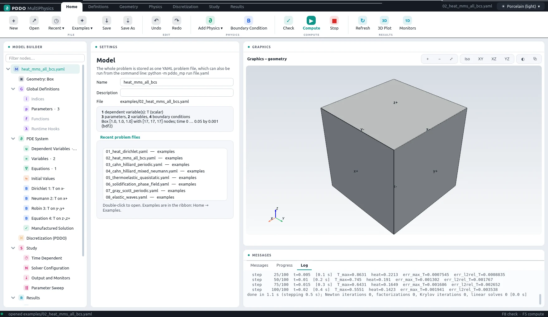
The complete problem file, examples/02_heat_mms_all_bcs.yaml

# Verification: nonlinear heat equation with a manufactured solution and every kind of
# boundary condition (time-dependent Dirichlet, Neumann, Robin, general equation).
# The engine derives the source terms and boundary data from the exact solution, so the
# reported errors measure the discretization error.
"k">name: heat_mms_all_bcs
"k">domain:
  "k">size: [1, 1, 1]
  "k">n: [17, 17, 17]
"k">parameters:
  "k">k0: 1.0
  "k">beta: 0.5
  "k">h: 2.0
"k">relations:
  "k">k: "k0*(1 + beta*T**2)"          # temperature-dependent conductivity
  "k">q: "-k*grad(T)"                   # heat flux
"k">fields:
  "k">T: scalar
"k">equations:
  "k">T: "dt(T) = -div(q)"
"k">boundary_conditions:
  - "k">faces: [x-]
    "k">T: {dirichlet: 0}                # value replaced by the exact data (manufactured mode)
  - "k">faces: [x+]
    "k">T: {neumann: 0}
  - "k">faces: [y-, y+]
    "k">T: {robin: [h, 1, 0]}            # h*T + dT/dn = g
  - "k">faces: [z-, z+]
    "k">T: {equation: "dot(q, n) = h*T"} # convective flux
"k">manufactured:
  "k">T: "1 + 0.5*sin(1.3*x + 0.4)*cos(0.9*y - 0.2)*exp(0.4*z)*exp(-t)"
"k">time:
  "k">end: 0.05
  "k">dt: 1.0e-3
  "k">scheme: bdf2
"k">output:
  "k">every: 50

**Figure 1.** The model in the GUI: the Model Builder tree on the left, the settings of the selected node in the middle, the graphics window on the right.

**Figure 2.** Variables: the conductivity and the heat flux as relations, used by the equation and by the boundary conditions.

**Figure 3.** A boundary condition written as an equation in the flux and the outward normal. The faces it acts on are highlighted in the graphics window.

**Figure 4.** The manufactured solution: the engine derives the source term and the boundary data from it.

3Results

Nodes: 17×17×17 = 4,913
PDDO order: 2, horizon 2.015 Δx
Time scheme: bdf2
Steps: 50 × Δt = 0.001
Newton iterations: 51
Factorizations: 1
Run time: 7 s

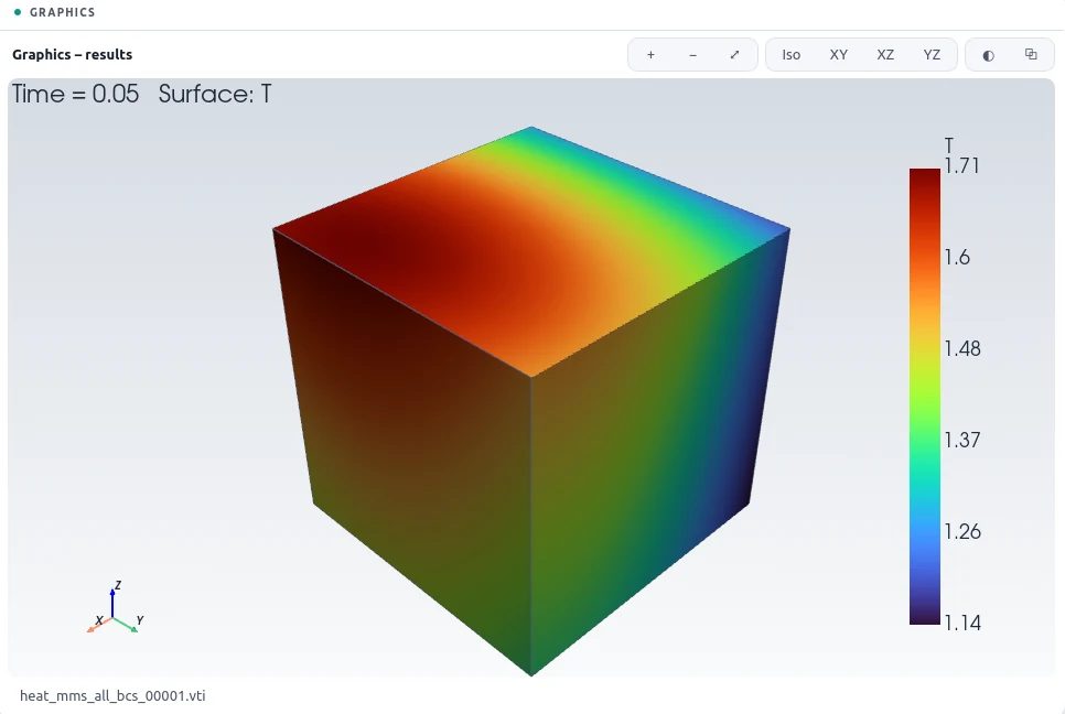
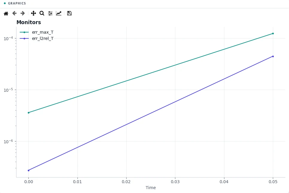
After 50 BDF2 steps the relative L2 error is 0.0045 % and the largest pointwise error 1.2×10^-4, on a grid of 17×17×17 nodes. The convergence study in the verification suite refines this grid and measures rates of 2.3 and 2.25: second order, including at the faces, edges and corners where the Robin and flux conditions act.

**Figure 5.** The computed temperature at the final time.

**Figure 6.** Relative L2 and largest error of T against time.

4Run It Yourself

The problem file ships with PDDO-MultiPhysics. Open it in the graphical interface and press Compute, or run it from the command line:

python -m pddo_mp gui examples/02_heat_mms_all_bcs.yaml
python -m pddo_mp run examples/02_heat_mms_all_bcs.yaml

Results go to results/heat_mms_all_bcs/ next to the problem file: a ParaView time series (.pvd), the monitors as CSV, and the final state. Any entry can be changed on the command line, for example --set time.end=0.025 for a run to half the end time. The user manual describes every part of the problem file and of the interface.

1The Problem

2The Problem File

3Results

4Run It Yourself

Have a coupled problem of your own?