Cahn-Hilliard in a bounded box | PDDO-MultiPhysics Examples

1The Problem

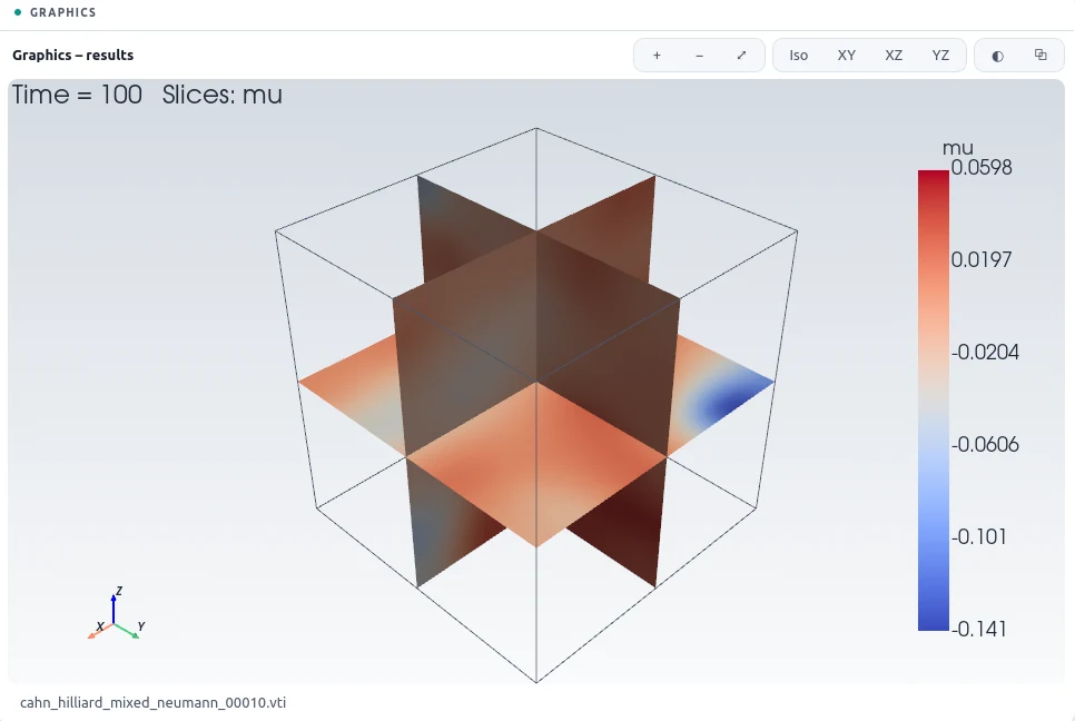
The same phase separation as in the periodic example, in a box with walls. Splitting the equation into composition c and chemical potential μ needs only second derivatives, and gives each field a natural boundary condition: a zero normal gradient of c (a 90° contact angle) and a zero normal gradient of μ (no flux through the wall).

$$\frac{\partial c}{\partial t} = \nabla\cdot(M\,\nabla\mu), \qquad \mu = f'(c) - \kappa\,\nabla^2 c$$

$$\nabla c\cdot\mathbf{n} = 0, \quad \nabla\mu\cdot\mathbf{n} = 0 \text{ on the walls}$$

2The Problem File

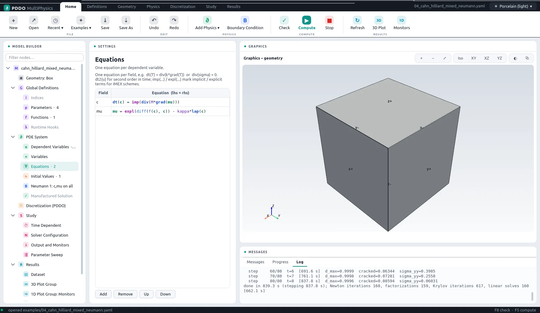
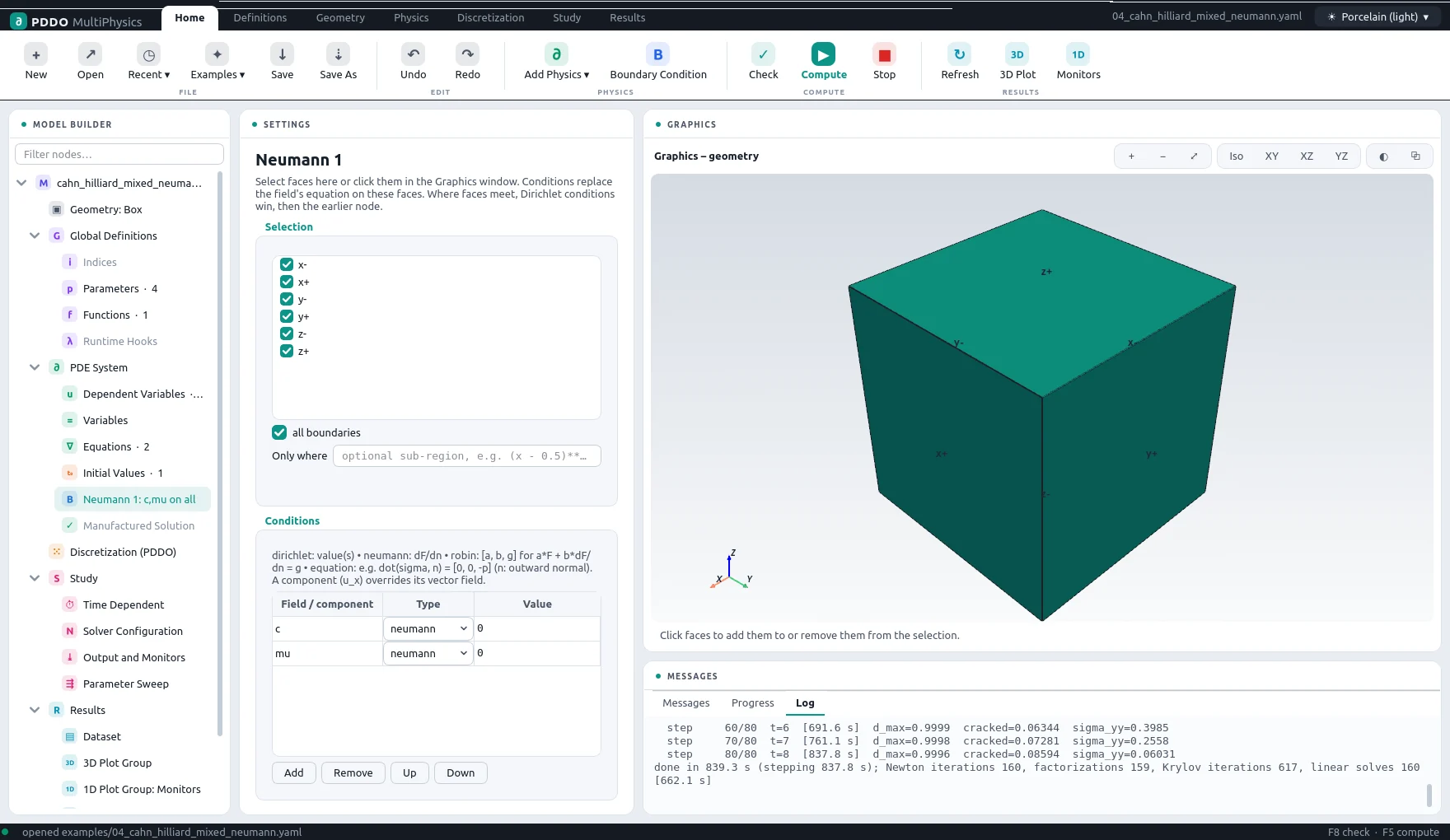
The chemical potential is a field with a stationary equation, mu = expl(diff(f(c), c)) - kappa*lap(c). With the nonlinear term explicit, the remaining system is linear with a constant matrix, set up once for the run. One boundary condition entry sets both fields on all faces.

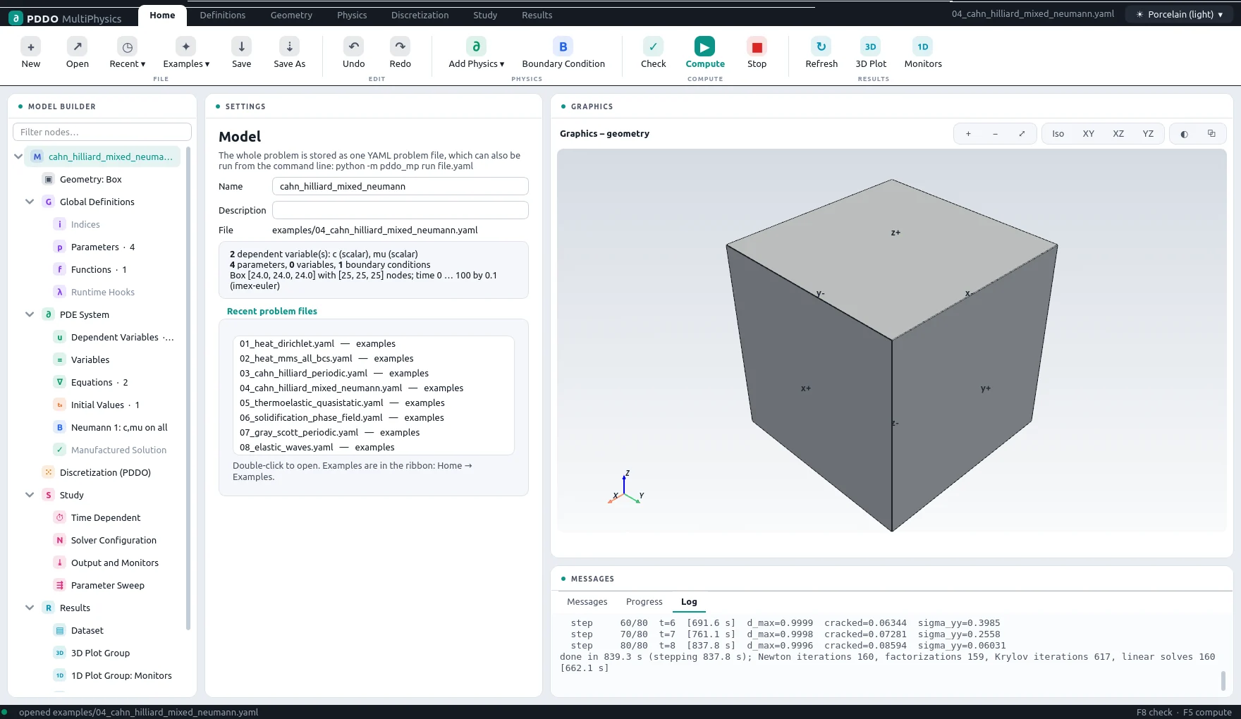
The complete problem file, examples/04_cahn_hilliard_mixed_neumann.yaml

# Cahn–Hilliard in mixed form on a bounded box (no periodicity):
#   dt(c) = div(M grad(mu)),   mu = f'(c) - kappa lap(c)
# Each field gets one boundary condition per face: dc/dn = 0 (contact angle 90°) and
# dmu/dn = 0 (no flux), so total mass is conserved. Only second derivatives are needed
# (PDDO order 2).
# Scheme: IMEX Euler with f'(c) explicit (expl) – the remaining system is linear with a
# constant matrix. Use "scheme: bdf2" and remove expl() for a fully implicit Newton solve.
"k">name: cahn_hilliard_mixed_neumann
"k">domain:
  "k">size: [24, 24, 24]
  "k">n: [25, 25, 25]
"k">parameters:
  "k">M: 1.0
  "k">kappa: 1.0
  "k">A: 1.0
  "k">c0: 0.5
"k">functions:
  "f(c)": "A*c**2*(1 - c)**2"
"k">fields:
  "k">c: scalar
  "k">mu: scalar
"k">equations:
  "k">c: "dt(c) = imp(div(M*grad(mu)))"
  "k">mu: "mu = expl(diff(f(c), c)) - kappa*lap(c)"
"k">boundary_conditions:
  - "k">faces: all
    "k">c: {neumann: 0}
    "k">mu: {neumann: 0}
"k">initial_conditions:
  "k">c: "c0 + 0.05*(rand() - 0.5)"
"k">seed: 2
"k">time:
  "k">end: 100
  "k">dt: 0.1
  "k">scheme: imex-euler
"k">output:
  "k">every: 100
"k">monitors:
  "k">mass: "mean(c)"
  "k">energy: "integral(f(c) + 0.5*kappa*dot(grad(c), grad(c)))"

**Figure 1.** The model in the GUI: the Model Builder tree on the left, the settings of the selected node in the middle, the graphics window on the right.

**Figure 2.** The mixed form: an evolution equation for c and a stationary equation for μ.

**Figure 3.** No-flux conditions for both fields on all faces.

3Results

Nodes: 25×25×25 = 15,625
PDDO order: 2, horizon 2.015 Δx
Time scheme: imex-euler
Steps: 1,000 × Δt = 0.1
Newton iterations: 1,001
Factorizations: 1
Run time: 6 min

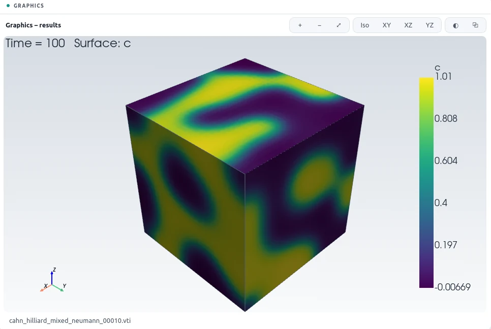
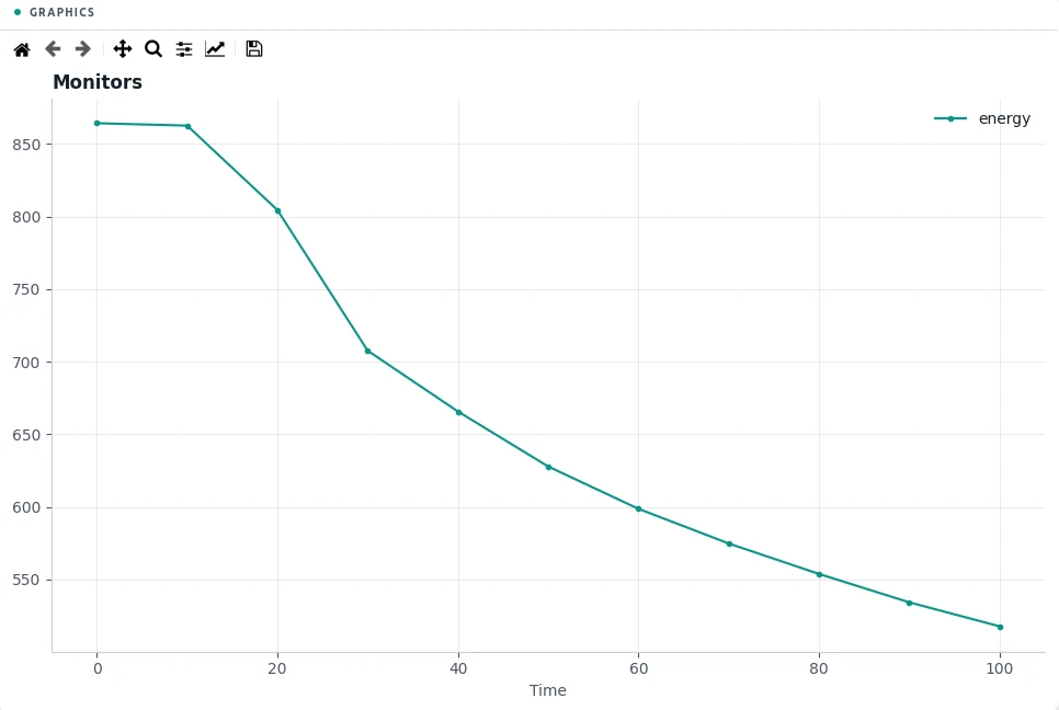
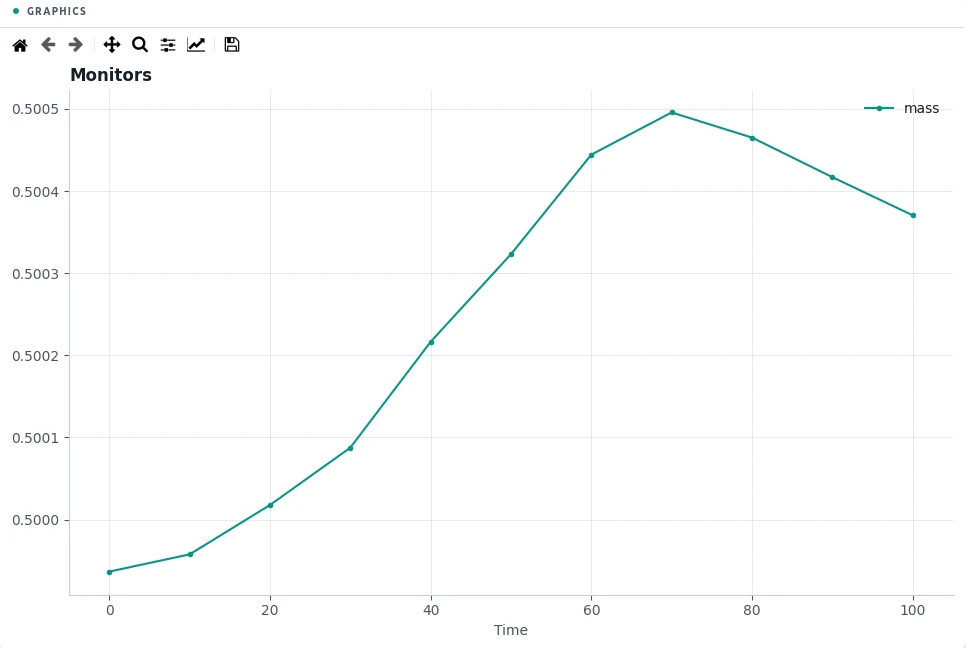
With no flux through the walls the mean composition stays at 0.4999, within 0.1 % over the run. At the wall nodes the no-flux conditions take the place of the equation, so on a bounded box mass is conserved to the accuracy of the discretization, not to round-off as in the periodic example. The free energy falls from 864 to 518 as the phases separate.

**Figure 4.** Composition at t = 100 in the bounded box.

**Figure 5.** The chemical potential μ on three slices.

**Figure 7.** Mean composition: constant.

4Run It Yourself

The problem file ships with PDDO-MultiPhysics. Open it in the graphical interface and press Compute, or run it from the command line:

python -m pddo_mp gui examples/04_cahn_hilliard_mixed_neumann.yaml
python -m pddo_mp run examples/04_cahn_hilliard_mixed_neumann.yaml

Results go to results/cahn_hilliard_mixed_neumann/ next to the problem file: a ParaView time series (.pvd), the monitors as CSV, and the final state. Any entry can be changed on the command line, for example --set time.end=50 for a run to half the end time. The user manual describes every part of the problem file and of the interface.

1The Problem

2The Problem File

3Results

4Run It Yourself

Have a coupled problem of your own?