Spinodal decomposition (Cahn-Hilliard) | PDDO-MultiPhysics Examples

1The Problem

A mixture quenched into its unstable range does not stay mixed: small fluctuations of composition grow, and the material separates into two phases that coarsen over time. The Cahn-Hilliard equation describes this with a double-well free energy and a gradient-energy term, which makes it fourth order in space. Composition is conserved, so its mean must not change.

$$\frac{\partial c}{\partial t} = M\,\nabla^2 f'(c) - M\kappa\,\nabla^4 c, \qquad f(c) = A\,c^2(1-c)^2$$

$$F = \int_\Omega f(c) + \tfrac{\kappa}{2}\,|\nabla c|^2 \; dV$$

2The Problem File

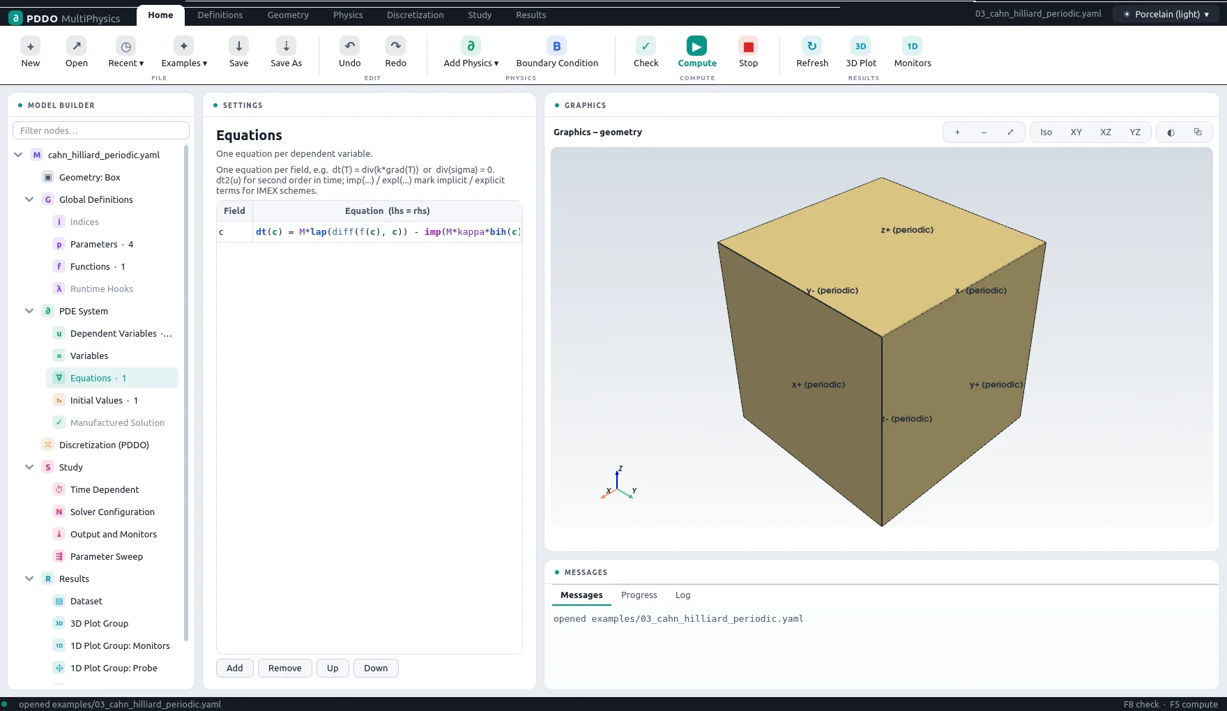
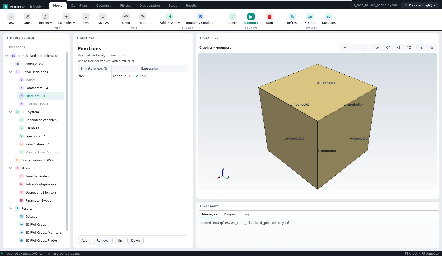
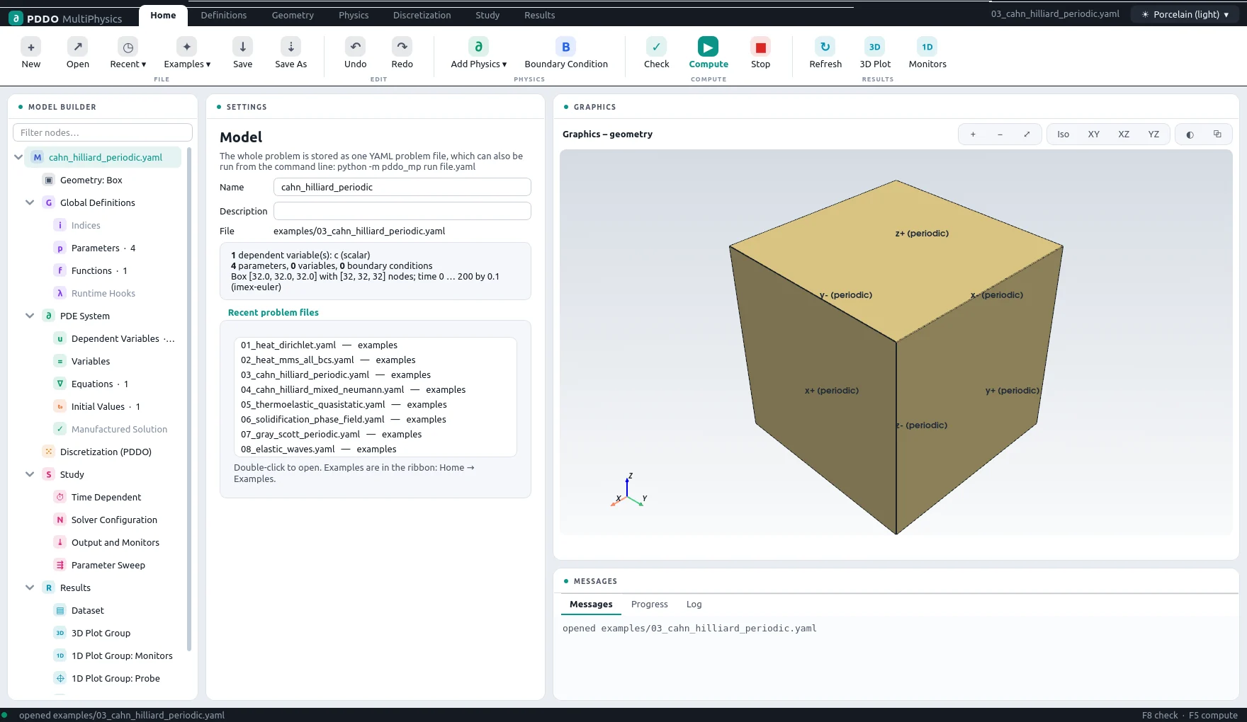
The equation is written as dt(c) = M*lap(diff(f(c), c)) - imp(M*kappa*bih(c)): diff differentiates the user function f(c), bih is the biharmonic operator, and imp() marks the term the IMEX scheme treats implicitly. The implicit operator is linear and constant, so its solver setup is reused for every step. The periodic box needs no boundary conditions.

The complete problem file, examples/03_cahn_hilliard_periodic.yaml

# Spinodal decomposition, periodic box, single-field Cahn–Hilliard (4th order).
#   dt(c) = M lap(f'(c)) - M kappa bih(c)
# Same semi-implicit split as crystal_growth_pddo: the biharmonic term is implicit (imp),
# the nonlinear term explicit, so the implicit operator I/dt + M kappa bih is constant and
# its solver setup is reused for every step.
"k">name: cahn_hilliard_periodic
"k">domain:
  "k">size: [32, 32, 32]
  "k">n: [32, 32, 32]
  "k">periodic: [true, true, true]
"k">parameters:
  "k">M: 1.0
  "k">kappa: 1.0
  "k">A: 1.0
  "k">c0: 0.4
"k">functions:
  "f(c)": "A*c**2*(1 - c)**2"
"k">fields:
  "k">c: scalar
"k">equations:
  "k">c: "dt(c) = M*lap(diff(f(c), c)) - imp(M*kappa*bih(c))"
"k">initial_conditions:
  "k">c: "c0 + 0.05*(rand() - 0.5)"
"k">seed: 1
"k">time:
  "k">end: 200
  "k">dt: 0.1
  "k">scheme: imex-euler
"k">output:
  "k">every: 200
"k">monitors:
  "k">mass: "mean(c)"
  "k">energy: "integral(f(c) + 0.5*kappa*dot(grad(c), grad(c)))"
  "k">c_min: "min(c)"
  "k">c_max: "max(c)"

**Figure 1.** The model in the GUI: the Model Builder tree on the left, the settings of the selected node in the middle, the graphics window on the right.

**Figure 2.** The single-field Cahn-Hilliard equation with the implicit biharmonic term.

**Figure 3.** The double-well free energy as a user function.

3Results

Nodes: 32×32×32 = 32,768
Periodic: xyz
PDDO order: 4, horizon 3.015 Δx
Time scheme: imex-euler
Steps: 2,000 × Δt = 0.1
Newton iterations: 2,000
Factorizations: 0
Run time: 6 min

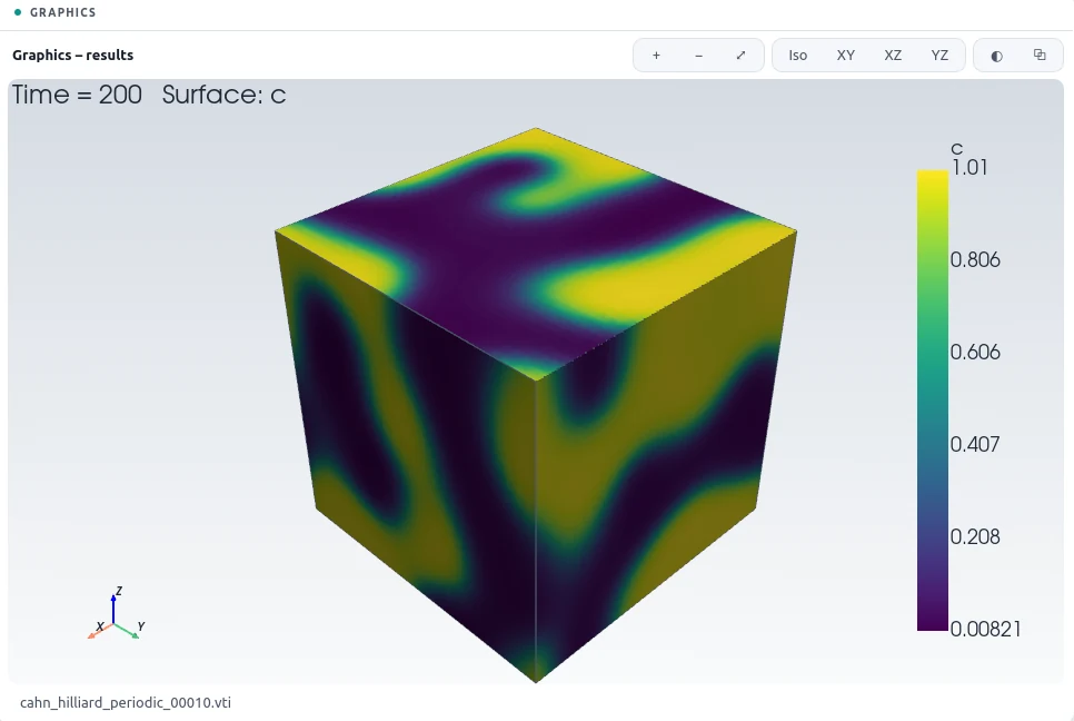
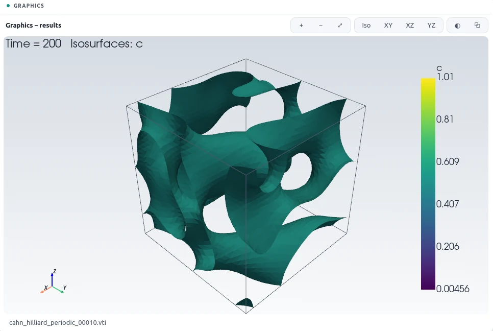
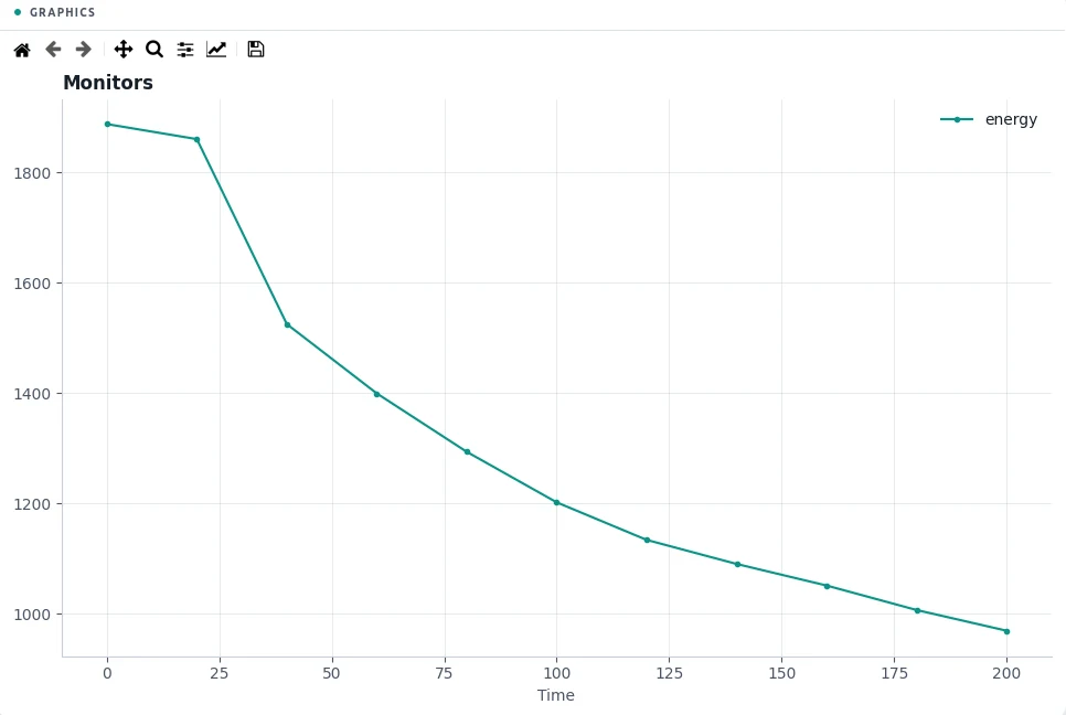
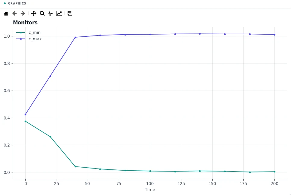
The mean composition starts at 0.4000 and changes by less than 1×10^-10 over 2000 steps: mass is conserved to round-off. The free energy falls from 1888 to 970 as the phases separate and coarsen, and the composition settles between 0.00456 and 1.01.

**Figure 4.** Composition c on the surface of the box at t = 200.

**Figure 5.** The c = 0.5 isosurface: two interpenetrating phases.

**Figure 7.** Smallest and largest composition: the two phases forming.

4Run It Yourself

The problem file ships with PDDO-MultiPhysics. Open it in the graphical interface and press Compute, or run it from the command line:

python -m pddo_mp gui examples/03_cahn_hilliard_periodic.yaml
python -m pddo_mp run examples/03_cahn_hilliard_periodic.yaml

Results go to results/cahn_hilliard_periodic/ next to the problem file: a ParaView time series (.pvd), the monitors as CSV, and the final state. Any entry can be changed on the command line, for example --set time.end=100 for a run to half the end time. The user manual describes every part of the problem file and of the interface.

1The Problem

2The Problem File

3Results

4Run It Yourself

Have a coupled problem of your own?