Solidification of an undercooled melt | PDDO-MultiPhysics Examples

1The Problem

A small solid sphere sits in a liquid cooled below its melting point. The solid grows into the liquid, and the latent heat it releases at the interface warms the surroundings, which in turn slows the growth. The phase field φ is 1 in the solid and 0 in the liquid; the temperature is dimensionless, with the melting point at 1 and the undercooled melt at 0.

$$\tau\,\frac{\partial\phi}{\partial t} = \epsilon^2\,\nabla^2\phi + \phi(1-\phi)\big(\phi - \tfrac12 + m(T)\big), \qquad m(T) = \frac{a}{\pi}\arctan\big(\gamma(T_{eq} - T)\big)$$

$$\frac{\partial T}{\partial t} = \nabla^2 T + K\,\frac{\partial\phi}{\partial t}$$

2The Problem File

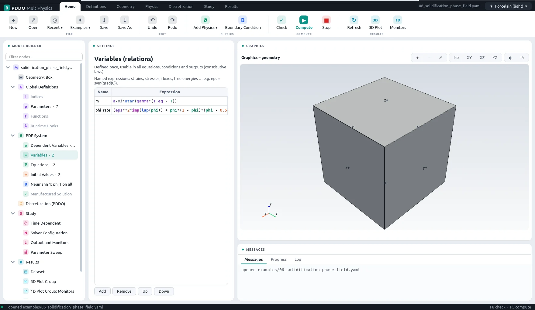
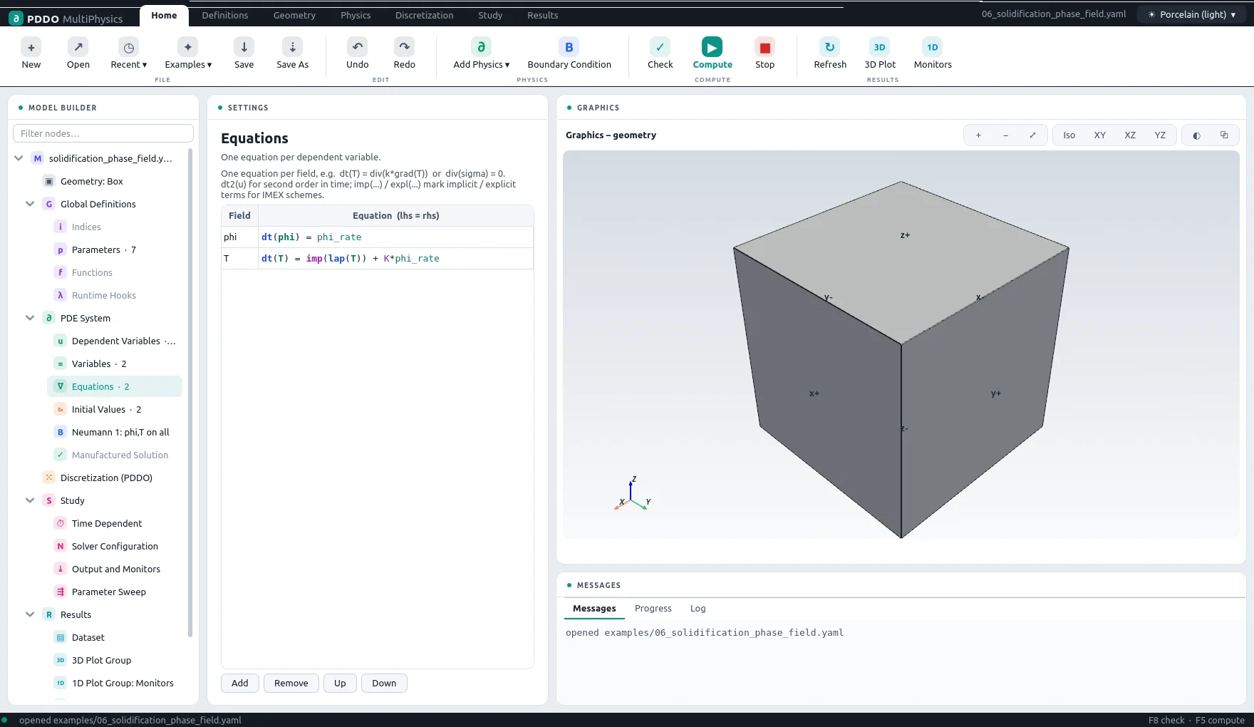
The rate of φ is written once as a relation, phi_rate, and used in both equations, so both have the form dt(f) = rhs. Diffusion is implicit and the reaction term explicit (IMEX Euler). The initial seed is a tanh profile around the centre of the box.

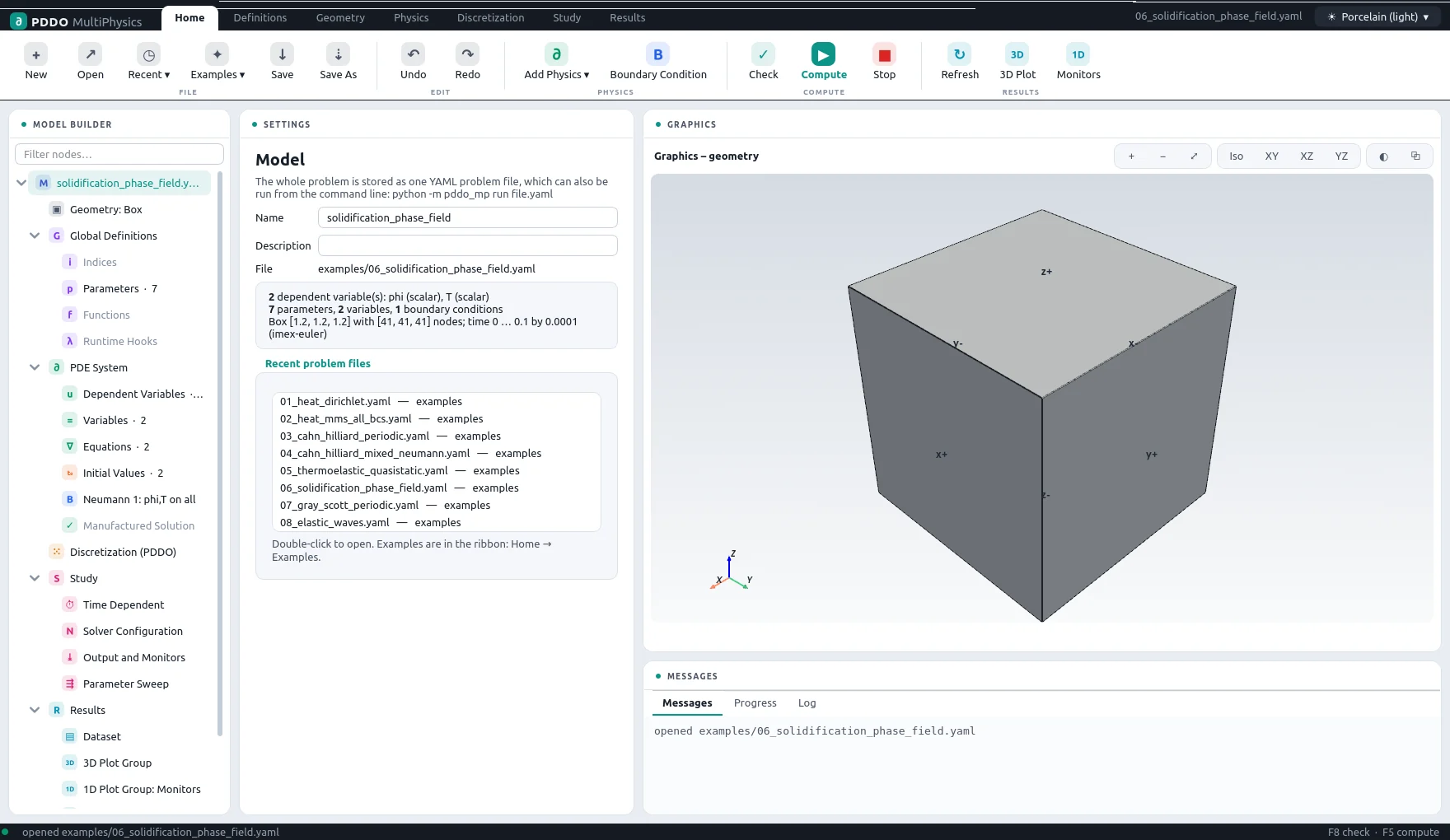
The complete problem file, examples/06_solidification_phase_field.yaml

# Solidification of an undercooled melt (Kobayashi-type phase field, isotropic, 3D):
#   tau dt(phi) = eps^2 lap(phi) + phi (1 - phi) (phi - 1/2 + m(T)),
#   m(T) = (a/pi) atan(gamma (T_eq - T))
#   dt(T) = lap(T) + K dt(phi)                (latent heat release)
# phi = 1 solid, 0 liquid; T is dimensionless (T_eq = 1, melt at T = 0).
# The rate of phi is written once as a relation and used in both equations, so both are
# of the form dt(f) = rhs. Diffusion is implicit (imp), the reaction explicit.
"k">name: solidification_phase_field
"k">domain:
  "k">size: [1.2, 1.2, 1.2]
  "k">n: [41, 41, 41]
"k">parameters:
  "k">tau: 3.0e-4
  "k">eps: 0.01
  "k">a: 0.9
  "k">gamma: 10.0
  "k">K: 1.6
  "k">T_eq: 1.0
  "k">r0: 0.08
"k">relations:
  "k">m: "a/pi*atan(gamma*(T_eq - T))"
  "k">phi_rate: "(eps**2*imp(lap(phi)) + phi*(1 - phi)*(phi - 0.5 + m))/tau"
"k">fields:
  "k">phi: scalar
  "k">T: scalar
"k">equations:
  "k">phi: "dt(phi) = phi_rate"
  "k">T: "dt(T) = imp(lap(T)) + K*phi_rate"
"k">boundary_conditions:
  - "k">faces: all
    "k">phi: {neumann: 0}
    "k">T: {neumann: 0}
"k">initial_conditions:
  # a solid seed in the centre of the box
  "k">phi: "0.5*(1 - tanh((sqrt((x - 0.6)**2 + (y - 0.6)**2 + (z - 0.6)**2) - r0)/(2*eps)))"
  "k">T: "0"
"k">time:
  "k">end: 0.1
  "k">dt: 1.0e-4
  "k">scheme: imex-euler
"k">output:
  "k">every: 100
"k">monitors:
  "k">solid_fraction: "mean(phi)"
  "k">T_max: "max(T)"

**Figure 1.** The model in the GUI: the Model Builder tree on the left, the settings of the selected node in the middle, the graphics window on the right.

**Figure 2.** The driving force m(T) and the phase-field rate as relations.

**Figure 3.** Phase field and heat equation, coupled through the rate of φ.

3Results

Nodes: 41×41×41 = 68,921
PDDO order: 2, horizon 2.015 Δx
Time scheme: imex-euler
Steps: 1,000 × Δt = 0.0001
Newton iterations: 1,000
Factorizations: 0
Run time: 21 min

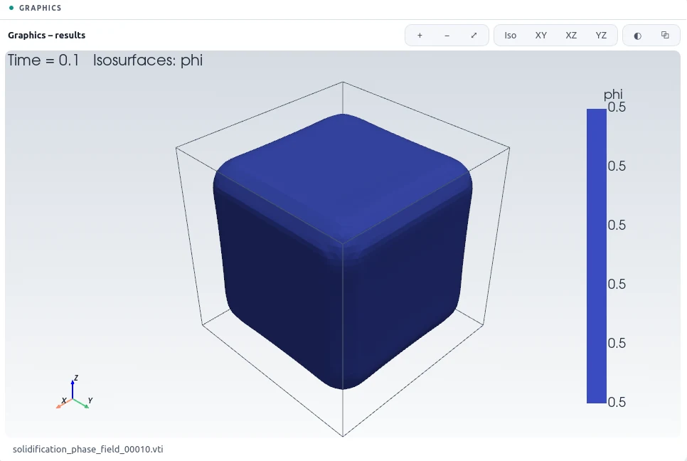
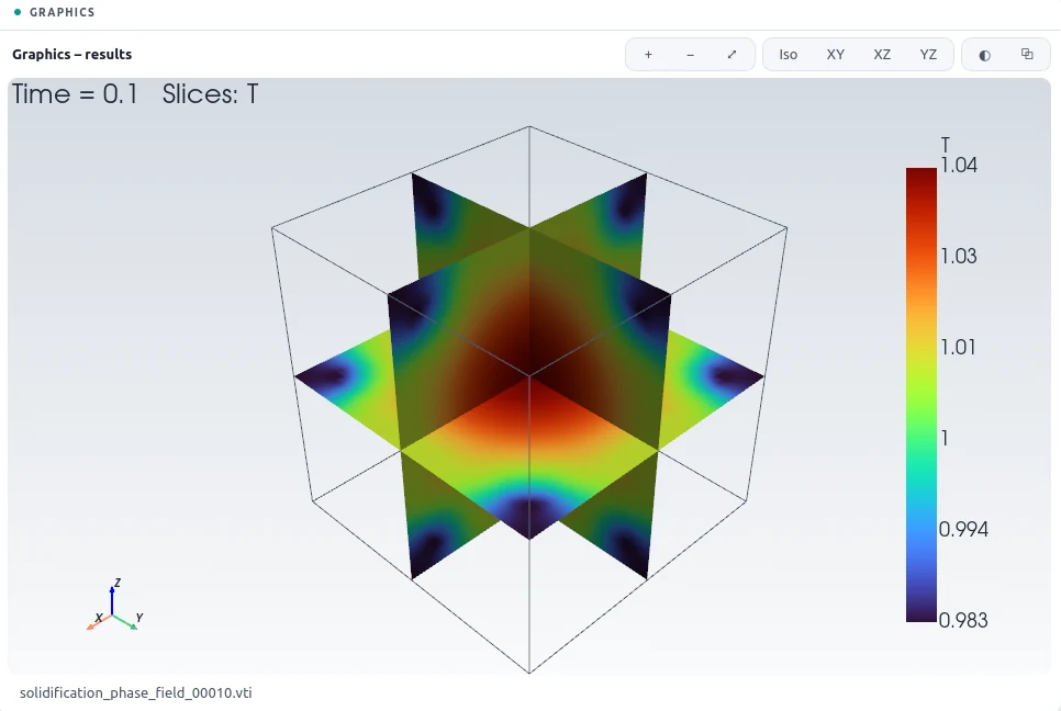
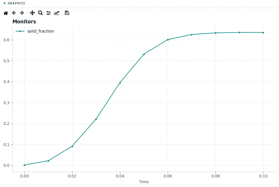
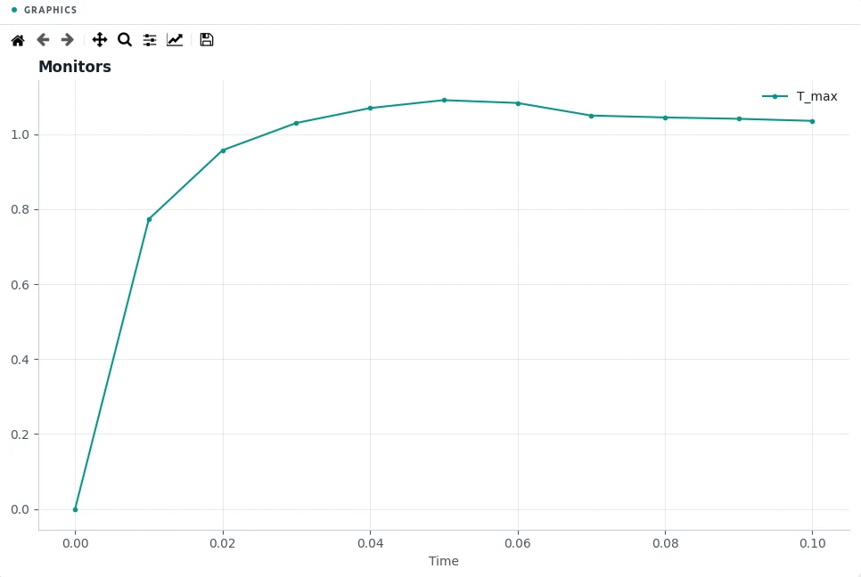
The solid fraction grows from 0.14 % to 63 % by t = 0.1. The released latent heat warms the melt next to the interface; the largest temperature reaches 1.04, close to the melting point, which is what limits the growth.

**Figure 4.** The solid-liquid interface (φ = 0.5) at the final time.

**Figure 5.** Temperature on three slices: the melt warmed by latent heat around the growing solid.

**Figure 6.** Solid fraction against time.

**Figure 7.** Largest temperature against time.

4Run It Yourself

The problem file ships with PDDO-MultiPhysics. Open it in the graphical interface and press Compute, or run it from the command line:

python -m pddo_mp gui examples/06_solidification_phase_field.yaml
python -m pddo_mp run examples/06_solidification_phase_field.yaml

Results go to results/solidification_phase_field/ next to the problem file: a ParaView time series (.pvd), the monitors as CSV, and the final state. Any entry can be changed on the command line, for example --set time.end=0.05 for a run to half the end time. The user manual describes every part of the problem file and of the interface.

1The Problem

2The Problem File

3Results

4Run It Yourself

Have a coupled problem of your own?