Elastic waves in a block | PDDO-MultiPhysics Examples

1The Problem

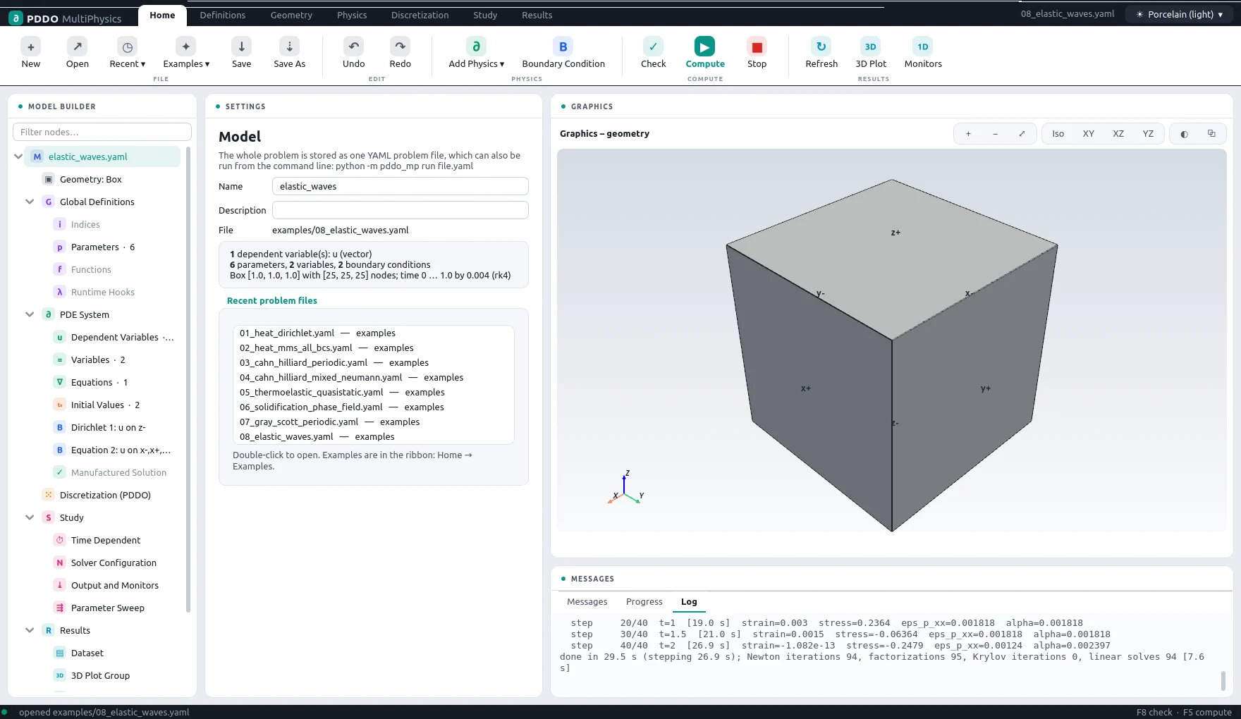
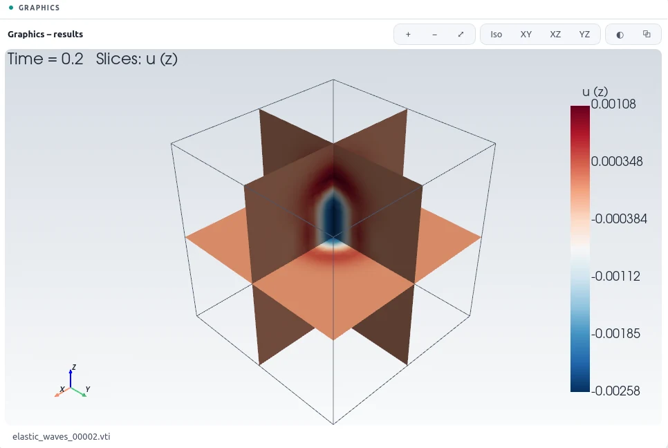
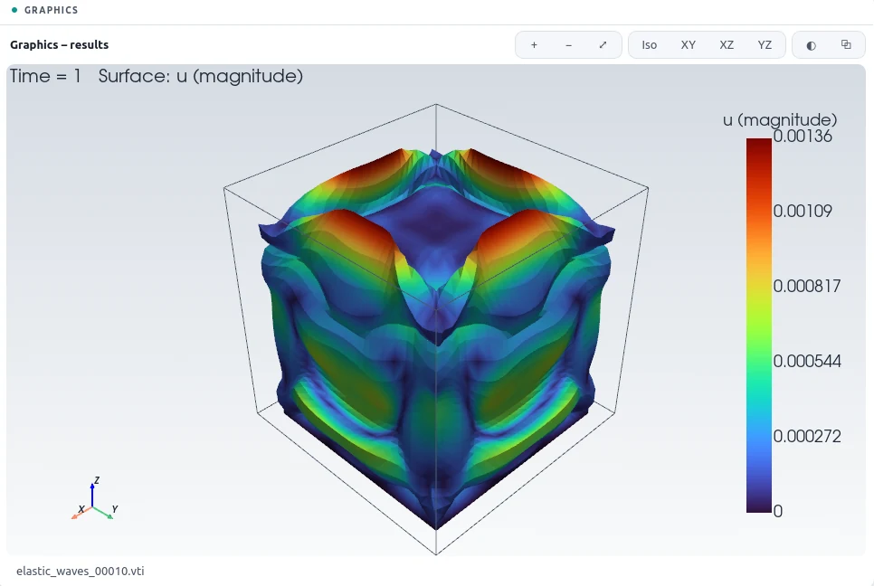
A Gaussian bump of vertical displacement is released at rest inside a unit block. It splits into pressure and shear waves that travel outwards, reflect from the free faces and the clamped base, and interfere. Without damping the total energy must stay constant, which makes it a clean check of the time integration.

$$\rho\,\frac{\partial^2 \mathbf{u}}{\partial t^2} = \nabla\cdot\boldsymbol{\sigma}, \qquad \boldsymbol{\sigma} = \lambda\,\mathrm{tr}(\boldsymbol{\varepsilon})\,\mathbf{I} + 2G\,\boldsymbol{\varepsilon}$$

$$E = \int_\Omega \tfrac12\,\boldsymbol{\sigma}:\boldsymbol{\varepsilon}\;dV + \int_\Omega \tfrac12\,\rho\,|\dot{\mathbf{u}}|^2\,dV$$

2The Problem File

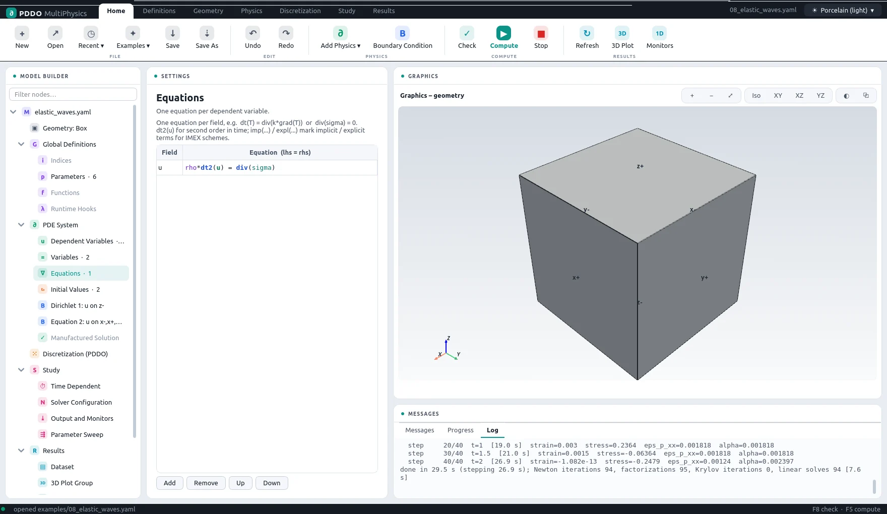
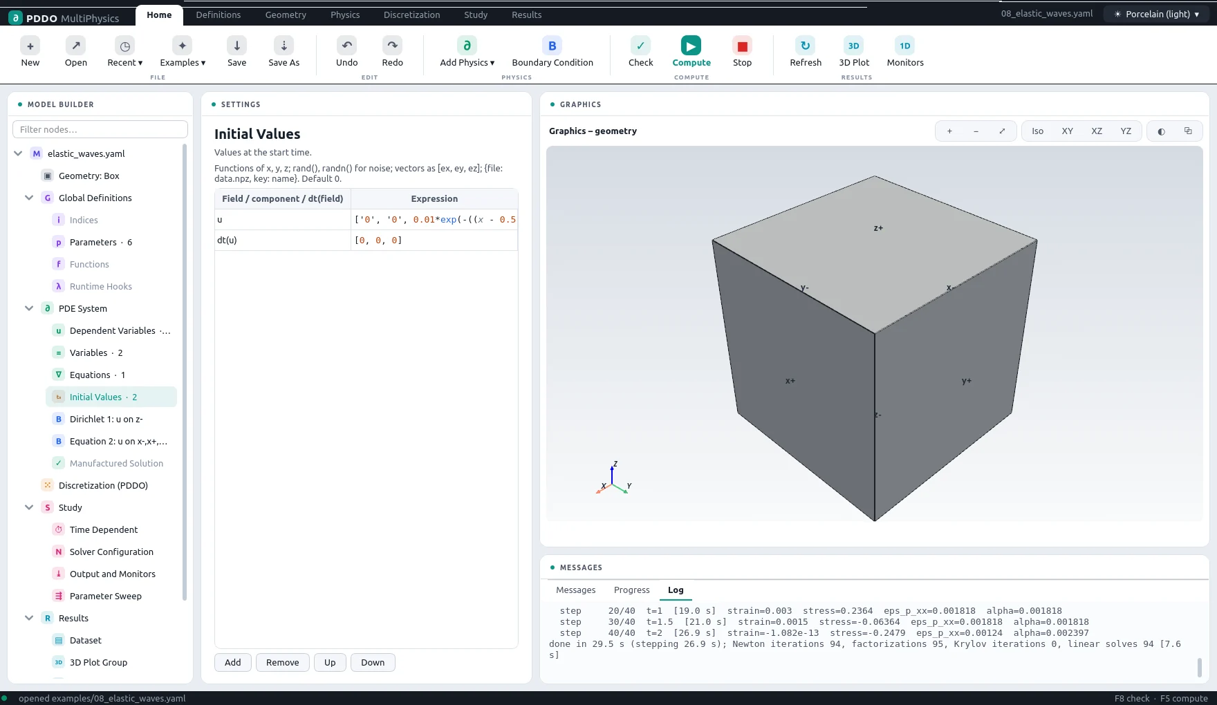
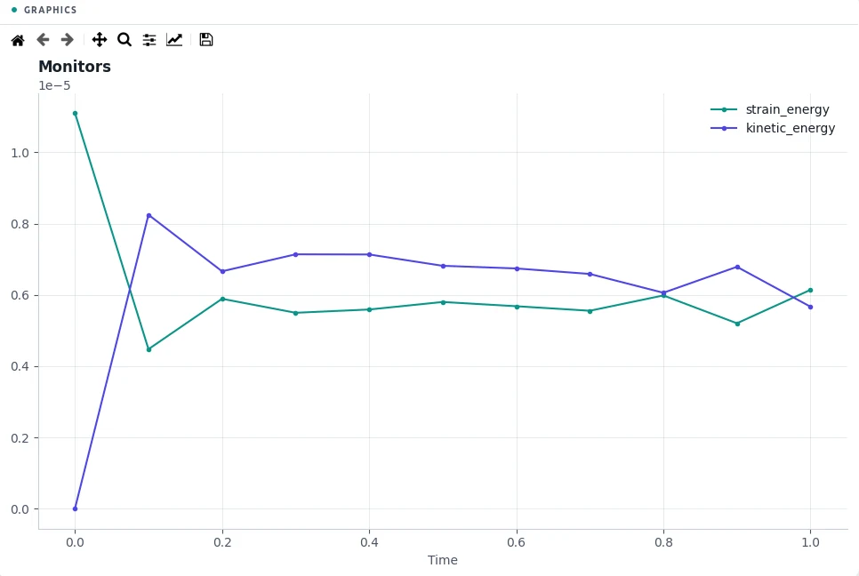
The equation is written with dt2(u); the engine rewrites it as a first-order system in u and its rate, and both need an initial condition (dt(u): [0, 0, 0]). The energies are monitors: integral(0.5*ddot(sigma, eps)) and integral(0.5*rho*dot(dt(u), dt(u))). The time scheme is the explicit fourth-order Runge-Kutta method; the stationary traction conditions on the free faces are solved at every stage.

The complete problem file, examples/08_elastic_waves.yaml

# Linear elastodynamics: rho dt2(u) = div(sigma), sigma = lambda tr(eps) I + 2 G eps.
# The second time derivative is rewritten automatically as a first-order system
# (u, u__t = dt(u)). A Gaussian displacement pulse is released at rest in a block whose
# bottom face is clamped; all other faces are traction free. Total energy is monitored
# (it should stay nearly constant).
"k">name: elastic_waves
"k">domain:
  "k">size: [1, 1, 1]
  "k">n: [25, 25, 25]
"k">parameters:
  "k">E: 1.0
  "k">nu: 0.25
  "k">rho: 1.0
  "k">lambda: "E*nu/((1 + nu)*(1 - 2*nu))"
  "k">G: "E/(2*(1 + nu))"
  "k">w: 0.08
"k">fields:
  "k">u: vector
"k">relations:
  "k">eps: "sym(grad(u))"
  "k">sigma: "lambda*tr(eps)*I + 2*G*eps"
"k">equations:
  "k">u: "rho*dt2(u) = div(sigma)"
"k">boundary_conditions:
  - "k">faces: [z-]
    "k">u: {dirichlet: [0, 0, 0]}
  - "k">faces: [x-, x+, y-, y+, z+]
    "k">u: {equation: "dot(sigma, n) = [0, 0, 0]"}
"k">initial_conditions:
  "k">u: ["0", "0", "0.01*exp(-((x - 0.5)**2 + (y - 0.5)**2 + (z - 0.6)**2)/w**2)"]
  "k">dt(u): [0, 0, 0]
"k">time:
  "k">end: 1.0
  "k">dt: 0.004
  "k">scheme: rk4
"k">output:
  "k">every: 25
  "k">fields: [u, sigma]
"k">monitors:
  "k">strain_energy: "integral(0.5*ddot(sigma, eps))"
  "k">kinetic_energy: "integral(0.5*rho*dot(dt(u), dt(u)))"
  "k">uz_max: "max(u_z)"

**Figure 1.** The model in the GUI: the Model Builder tree on the left, the settings of the selected node in the middle, the graphics window on the right.

**Figure 2.** The wave equation with the second time derivative dt2(u).

Initial values: the Gaussian pulse in uz and zero initial velocity. — **Figure 3.** Initial values: the Gaussian pulse in u_z and zero initial velocity.

3Results

Nodes: 25×25×25 = 15,625
PDDO order: 2, horizon 2.015 Δx
Time scheme: rk4
Steps: 250 × Δt = 0.004
Newton iterations: 1,001
Factorizations: 1
Run time: 116 s

The initial strain energy is 1.11×10^-5. As the pulse spreads, energy moves back and forth between strain and motion, the kinetic energy peaking at 8.25×10^-6. Their sum is not exactly constant: it rises by 15 % in the first tenth of the run, while the pulse — only about two node spacings wide — breaks up into waves the grid resolves, and then stays within 7 % of that level, drifting slowly down (-7 % by the end). The jump is a resolution effect: with the pulse twice as wide (--set parameters.w=0.16) it falls to 5 %. Use a pulse several node spacings wide, or a finer grid, when the energy balance matters.

Vertical displacement uz on three slices, early in the run: the pulse spreading out. — **Figure 4.** Vertical displacement u_z on three slices, early in the run: the pulse spreading out.

**Figure 5.** Displacement magnitude on the deformed block at the final time, after reflections.

**Figure 6.** Strain and kinetic energy against time: energy moves between the two.

4Run It Yourself

The problem file ships with PDDO-MultiPhysics. Open it in the graphical interface and press Compute, or run it from the command line:

python -m pddo_mp gui examples/08_elastic_waves.yaml
python -m pddo_mp run examples/08_elastic_waves.yaml

Results go to results/elastic_waves/ next to the problem file: a ParaView time series (.pvd), the monitors as CSV, and the final state. Any entry can be changed on the command line, for example --set time.end=0.5 for a run to half the end time. The user manual describes every part of the problem file and of the interface.

1The Problem

2The Problem File

3Results

4Run It Yourself

Have a coupled problem of your own?