1The Problem
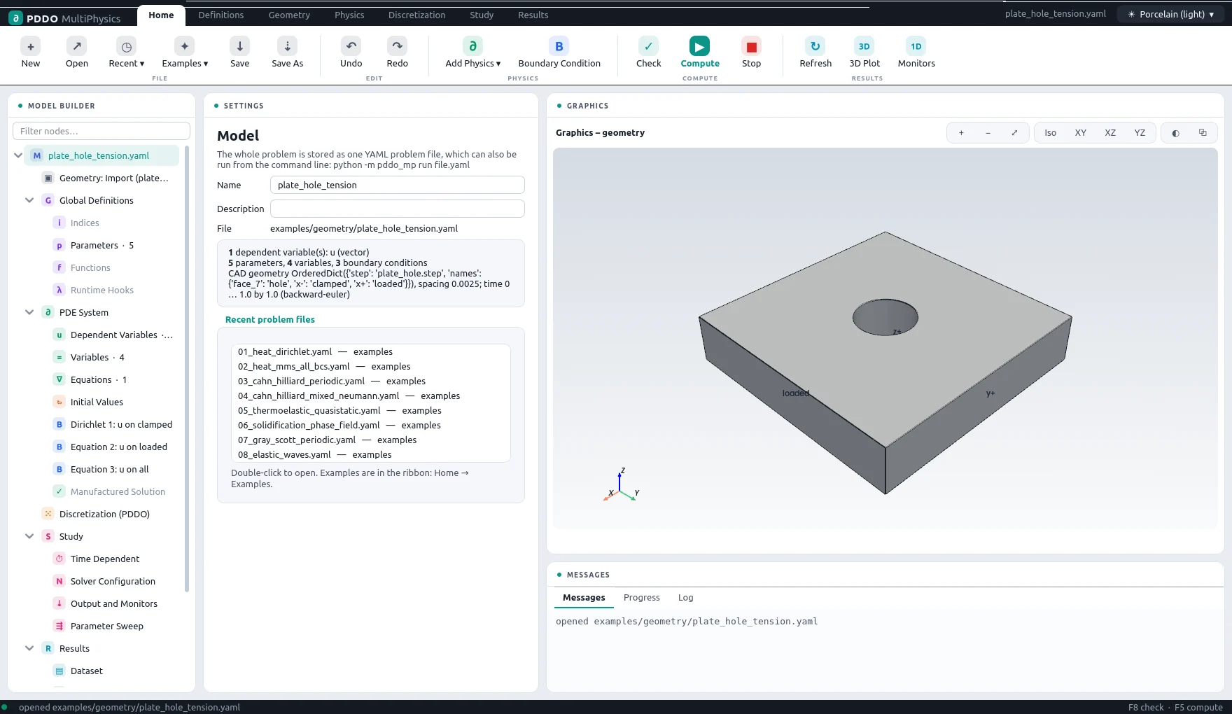
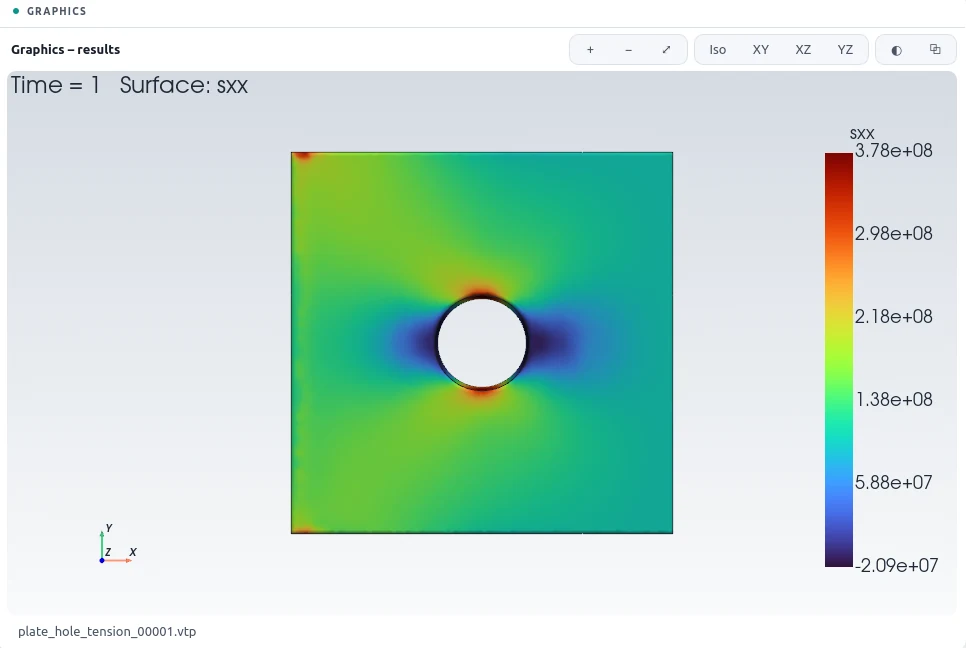
The plate is 100×100×20 mm with a 25 mm hole through its centre. One end is clamped and the other carries a uniform traction of 100 MPa. The stress peaks at the sides of the hole, and capturing that peak needs a fine discretization there, but not across the whole plate.
2The Problem File
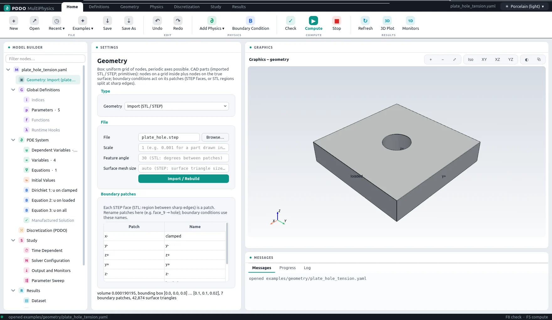
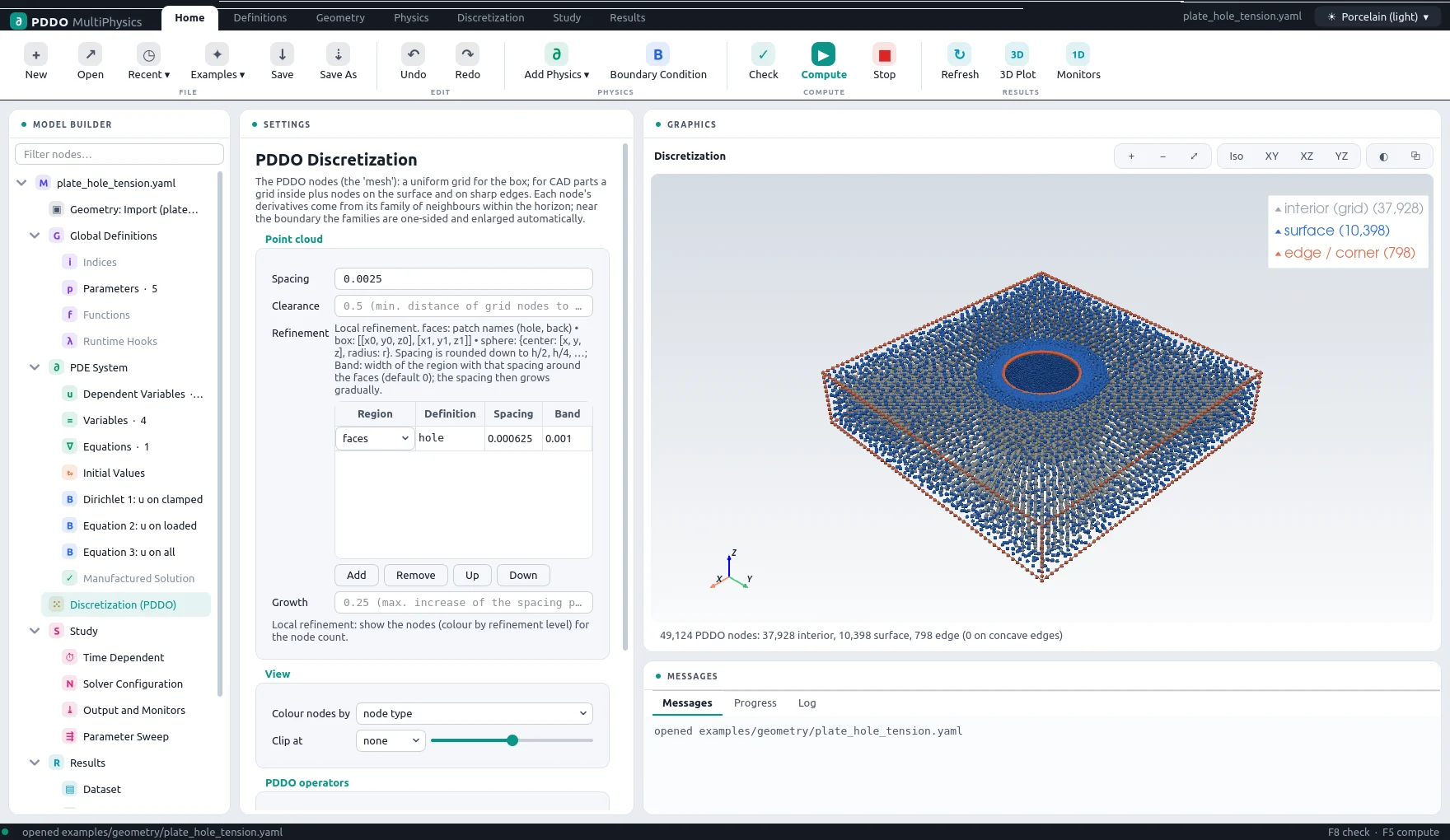
The base spacing is 2.5 mm. A refine entry asks for 0.625 mm nodes
within 1 mm of the face named hole; the spacing grades smoothly between the two.
The rest is linear elasticity with the stress component sxx = sigma[0, 0] and the von
Mises stress as relations for output.
The complete problem file, examples/geometry/plate_hole_tension.yaml
# Stress concentration at a hole: steel plate 100 x 100 x 20 mm with a 25 mm hole, clamped on
# one end and pulled with 100 MPa on the other. Local refinement: 2.5 mm nodes in the plate,
# 0.625 mm nodes around the hole (graded in between) – a fraction of the nodes of a uniform
# 0.625 mm cloud. Compare the peak stress at the hole with `--set domain.refine=[]`.
"k">name: plate_hole_tension
"k">domain:
  "k">type: geometry
  "k">geometry:
    "k">step: plate_hole.step
    "k">names: {face_7: hole, x-: clamped, x+: loaded}
  "k">spacing: 0.0025
  "k">refine:
    - "k">faces: [hole]
      "k">spacing: 0.000625
      "k">distance: 0.001
"k">parameters:
  "k">E: 210.0e9
  "k">nu: 0.3
  "k">p: 100.0e6
  "k">lambda: "E*nu/((1 + nu)*(1 - 2*nu))"
  "k">G: "E/(2*(1 + nu))"
"k">fields:
  "k">u: vector
"k">relations:
  "k">eps: "sym(grad(u))"
  "k">sigma: "lambda*tr(eps)*I + 2*G*eps"
  "k">sxx: "sigma[0, 0]"
  "k">von_mises: "sqrt(3/2*ddot(dev(sigma), dev(sigma)))"
"k">equations:
  "k">u: "div(sigma) = 0"
"k">boundary_conditions:
  - "k">faces: [clamped]
    "k">u: {dirichlet: [0, 0, 0]}
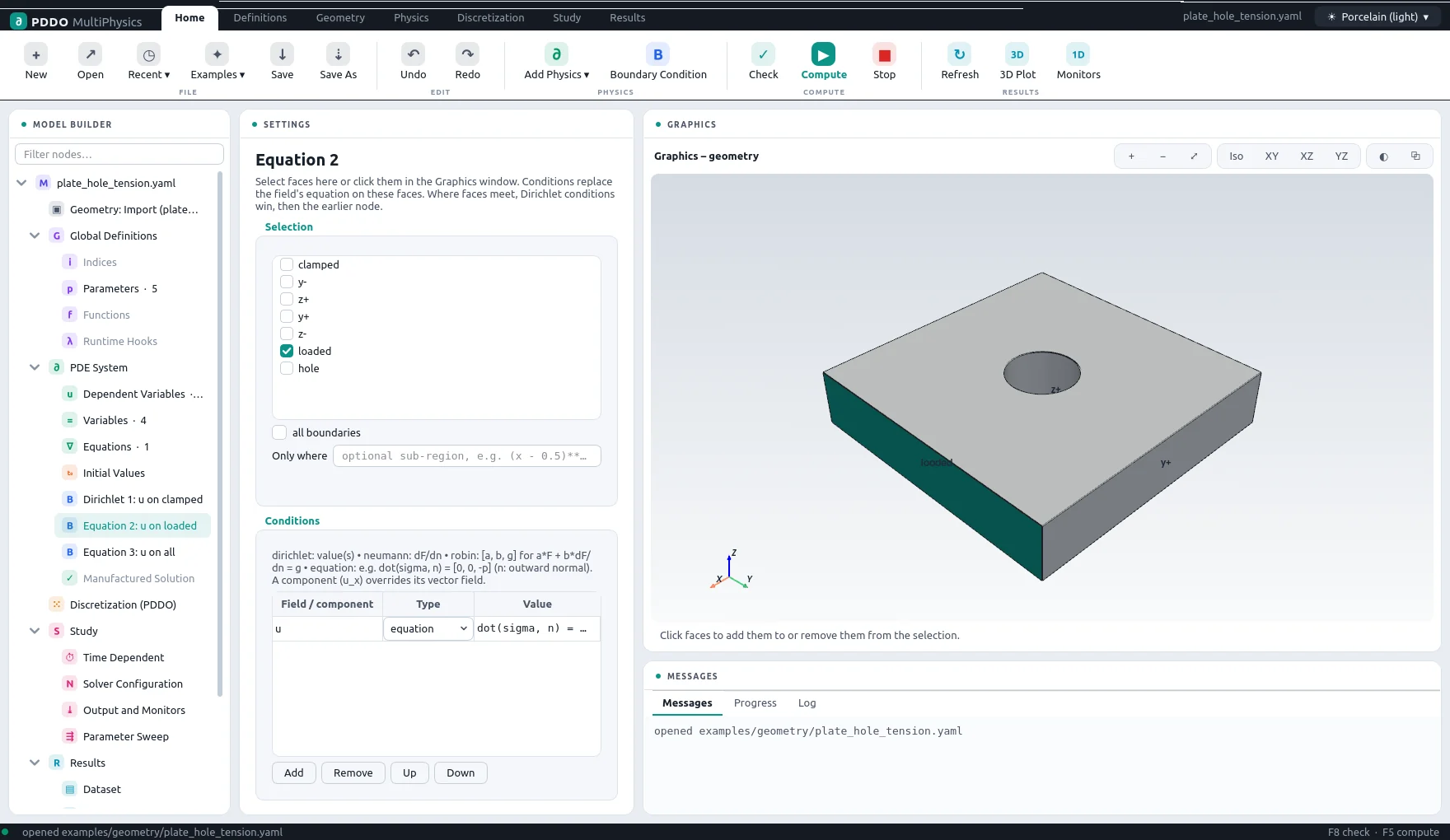
  - "k">faces: [loaded]
    "k">u: {equation: "dot(sigma, n) = [p, 0, 0]"}
  - "k">faces: all
    "k">u: {equation: "dot(sigma, n) = [0, 0, 0]"}
"k">time:
  "k">end: 1.0
  "k">dt: 1.0
  "k">scheme: backward-euler
"k">output:
  "k">every: 1
  "k">fields: [u, sxx, von_mises]
"k">monitors:
  "k">sxx_max: "max(sxx)"
  "k">vm_max: "max(von_mises)"
  "k">u_max: "max(sqrt(dot(u, u)))"
3Discretization
The refined cloud has 49,124 nodes, a fraction of what a uniform 0.625 mm cloud would need. The refinement region is drawn in the node view.
It is still the heaviest example here: the 147,000-unknown system of the order-2 stencil has 86 million nonzeros, too many to factorize, so the solver uses ILU-preconditioned GMRES (838 iterations). Most of the run time goes to that single linear solve.
4Results
- Nodes
- 49,124 (point cloud)
- PDDO order
- 2, horizon 2.015 Δx
- Time scheme
- backward-euler
- Steps
- 1 × Δt = 1
- Newton iterations
- 1
- Factorizations
- 0
- Run time
- 78 min
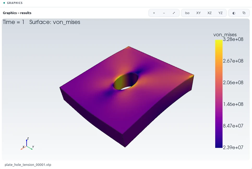
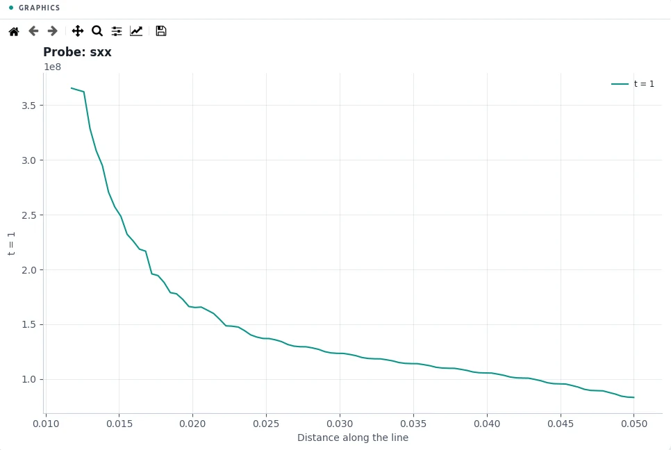
The largest axial stress is 379 MPa, 3.79 times the
applied traction, at the sides of the hole. The largest von Mises stress is 372 MPa and the
largest displacement 121 µm. Running the same file with --set domain.refine=[]
shows how much of the peak a uniform 2.5 mm cloud misses.
5Run It Yourself
The problem file ships with PDDO-MultiPhysics. Open it in the graphical interface and press Compute, or run it from the command line:
python -m pddo_mp gui examples/geometry/plate_hole_tension.yaml
python -m pddo_mp run examples/geometry/plate_hole_tension.yaml
Results go to results/plate_hole_tension/
next to the problem file: a ParaView time series (.pvd), the monitors as CSV, and the
final state. Any entry can be changed on the command line, for example
--set domain.spacing=0.005 for a coarser, faster run. The user manual
describes every part of the problem file and of the interface.