1The Problem
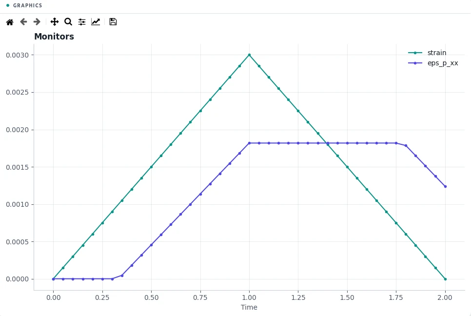
A bar in uniaxial tension is stretched to three times the yield strain and then brought back to zero length, which drives it through elastic loading, plastic flow with hardening, elastic unloading and reverse yielding. In uniaxial stress the exact response is known, so the computed stress can be compared with it at every step.
2The Problem File
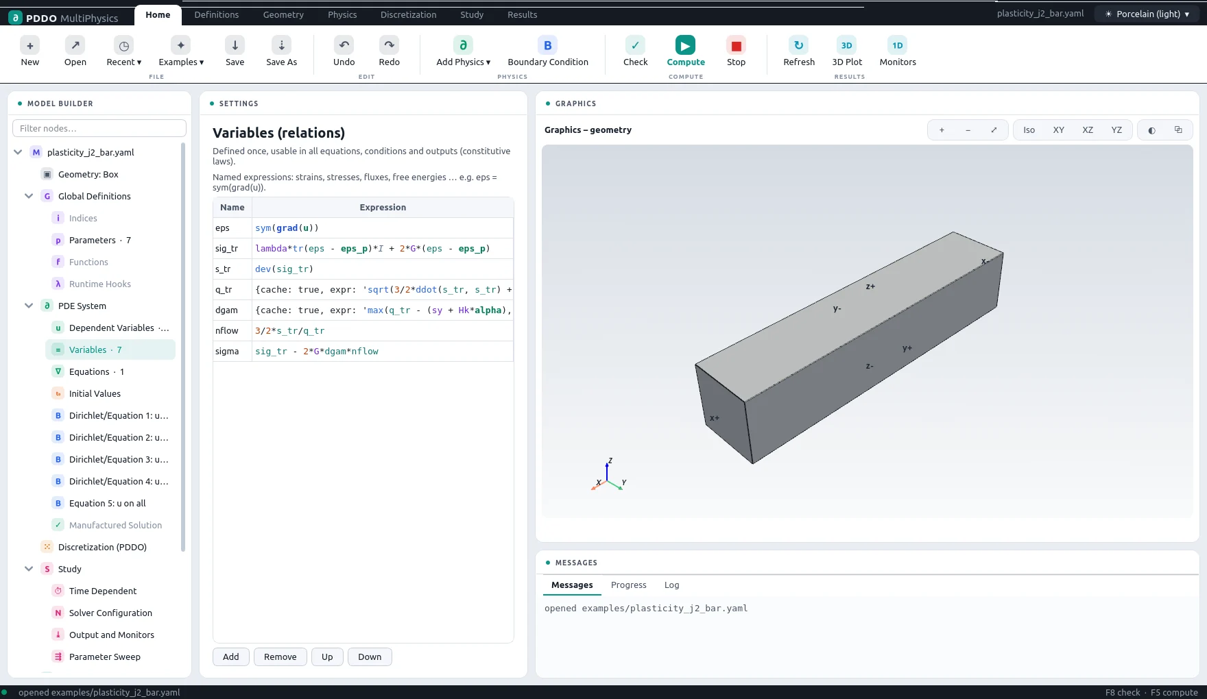
For linear hardening the radial return has a closed form, so the stress can be written as
a function of the current strain and of the plastic state at the start of the step. The plastic
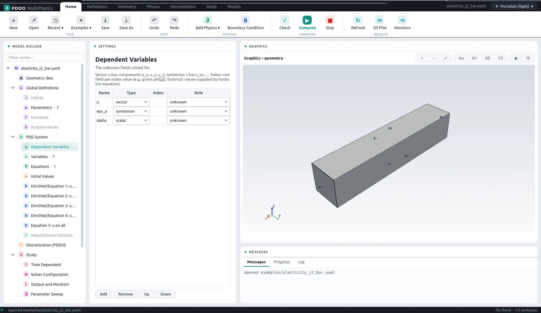
strain and the hardening variable are fields with an update rule, applied once per
converged step: eps_p: {type: symtensor, update: "eps_p + dgam*nflow"}. Because Newton
differentiates the returned stress exactly, it uses the consistent tangent and converges
quadratically. The intermediate q_tr and dgam are marked
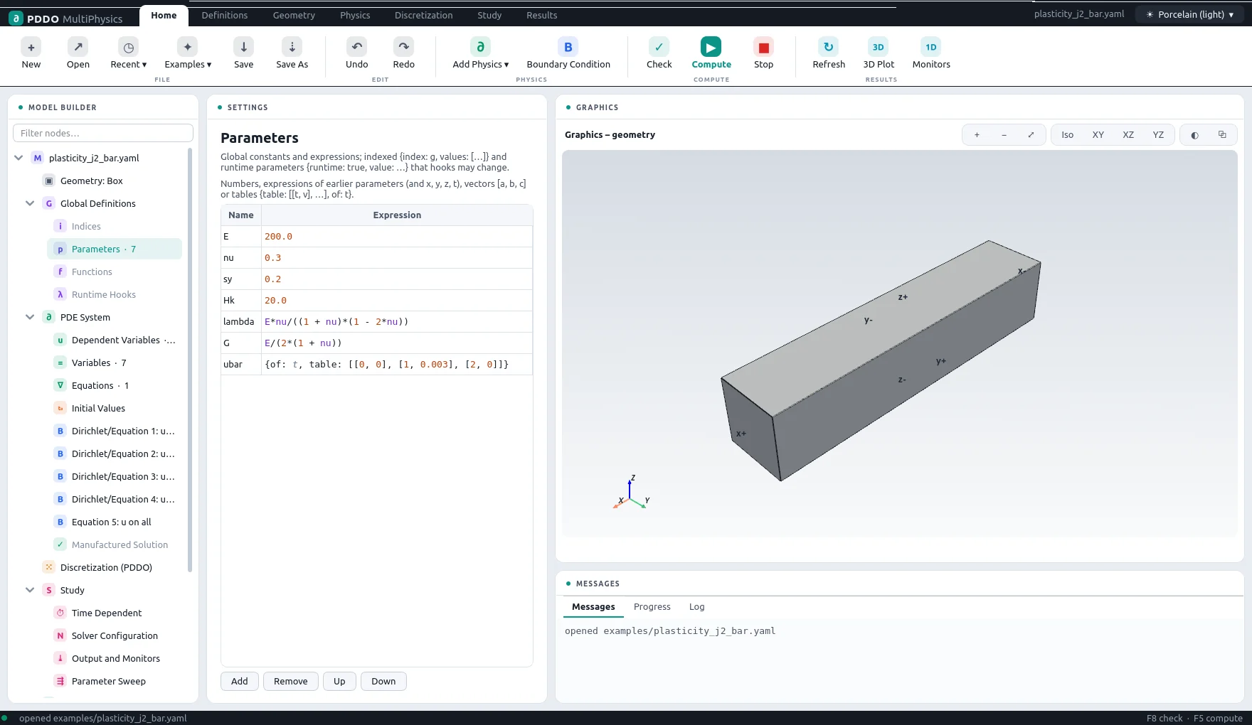
cache: true, which keeps the symbolic derivatives small. The load path is a table of the
end displacement against time.
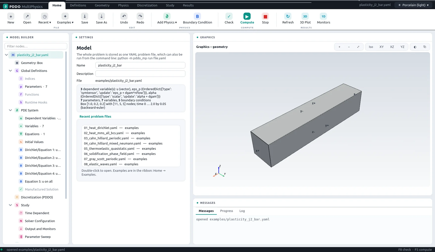
The complete problem file, examples/plasticity_j2_bar.yaml
# J2 plasticity (small strain, linear isotropic hardening) - bar in uniaxial tension,
# loaded to 3x the yield strain and unloaded.
# Monolithic return mapping: for linear hardening the radial return has a closed form, so
# the stress is written as a function of the current strain and the plastic state at the
# start of the step (eps_p, alpha):
#   trial stress  sig_tr = C : (eps - eps_p),  q_tr = von Mises(sig_tr)
#   dgam = <q_tr - (sy + Hk alpha)> / (3 G + Hk),   sigma = sig_tr - 2 G dgam nflow
# Newton differentiates sigma exactly: the consistent (algorithmic) tangent, quadratic
# convergence. The internal variables eps_p, alpha are update-rule fields, updated once per
# converged step with the same closed form. q_tr and dgam are cached (evaluated pointwise):
# much smaller symbolic derivatives. (A staggered alternative: the trial stress in
# div(sigma) with solver.staggered iterations - linear convergence, see README.)
# Uniaxial analytic curve: sigma = E eps up to sigma_y, then sigma_y + E H/(E + H) (eps - eps_y).
"k">name: plasticity_j2_bar
"k">domain:
  "k">size: [1.0, 0.2, 0.2]
  "k">n: [11, 5, 5]
"k">parameters:
  "k">E: 200.0
  "k">nu: 0.3
  "k">sy: 0.2                         # yield stress (eps_y = 1e-3)
  "k">Hk: 20.0                        # isotropic hardening modulus
  "k">lambda: "E*nu/((1 + nu)*(1 - 2*nu))"
  "k">G: "E/(2*(1 + nu))"
  "k">ubar: {table: [[0, 0], [1, 3.0e-3], [2, 0]], of: t}     # end displacement (load path)
"k">fields:
  "k">u: vector
  "k">eps_p: {type: symtensor, update: "eps_p + dgam*nflow"}
  "k">alpha: {type: scalar, update: "alpha + dgam"}
"k">relations:
  "k">eps: "sym(grad(u))"
  "k">sig_tr: "lambda*tr(eps - eps_p)*I + 2*G*(eps - eps_p)"   # trial (elastic predictor)
  "k">s_tr: "dev(sig_tr)"
  "k">q_tr: {expr: "sqrt(3/2*ddot(s_tr, s_tr) + 1e-24)", cache: true}   # von Mises (smooth at 0)
  "k">dgam: {expr: "max(q_tr - (sy + Hk*alpha), 0)/(3*G + Hk)", cache: true}   # plastic multiplier
  "k">nflow: "3/2*s_tr/q_tr"                                   # flow direction
  "k">sigma: "sig_tr - 2*G*dgam*nflow"                         # return-mapped stress
"k">equations:
  "k">u: "div(sigma) = 0"
"k">boundary_conditions:
  - "k">faces: [x-]
    "k">u: {equation: "dot(sigma, n) = [0, 0, 0]"}
    "k">u_x: {dirichlet: 0}
  - "k">faces: [y-]
    "k">u: {equation: "dot(sigma, n) = [0, 0, 0]"}
    "k">u_y: {dirichlet: 0}
  - "k">faces: [z-]
    "k">u: {equation: "dot(sigma, n) = [0, 0, 0]"}
    "k">u_z: {dirichlet: 0}
  - "k">faces: [x+]
    "k">u: {equation: "dot(sigma, n) = [0, 0, 0]"}
    "k">u_x: {dirichlet: "ubar"}
  - "k">faces: all
    "k">u: {equation: "dot(sigma, n) = [0, 0, 0]"}
"k">time:
  "k">end: 2.0
  "k">dt: 0.05
  "k">scheme: backward-euler
"k">output:
  "k">every: 10
"k">monitors:
  "k">strain: "mean(eps[0, 0])"
  "k">stress: "mean(sigma[0, 0])"
  "k">eps_p_xx: "mean(eps_p_xx)"
  "k">alpha: "max(alpha)"
3Results
- Nodes
- 11×5×5 = 275
- PDDO order
- 2, horizon 2.015 Δx
- Time scheme
- backward-euler
- Steps
- 40 × Δt = 0.05
- Newton iterations
- 94
- Factorizations
- 95
- Run time
- 23 s
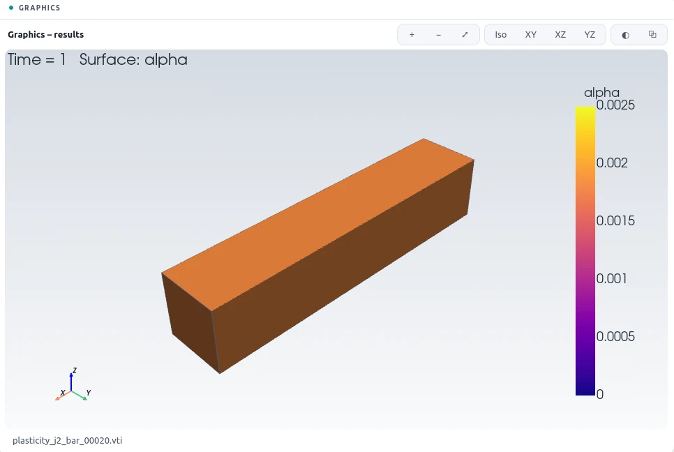
This run stored every output step for the plots: --set output.every=1 --set "output.fields=[u, eps_p, alpha]" on the command line; the problem file itself writes less often.
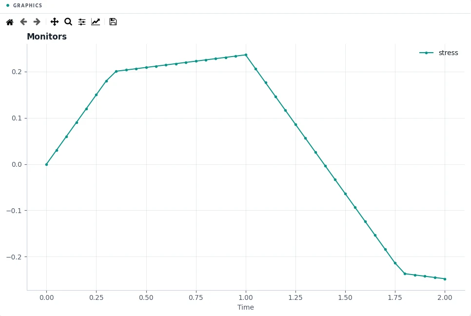
The stress peaks at 0.2364 at the largest stretch and reaches -0.2479 after reverse yielding at the end of unloading. Replaying the uniaxial return mapping over the same strain history, the largest difference from the computed stress is 1.2×10⁻⁹ of the peak. Newton needed 2.4 iterations per load step on average.
4Run It Yourself
The problem file ships with PDDO-MultiPhysics. Open it in the graphical interface and press Compute, or run it from the command line:
python -m pddo_mp gui examples/plasticity_j2_bar.yaml
python -m pddo_mp run examples/plasticity_j2_bar.yaml --set output.every=1 --set "output.fields=[u, eps_p, alpha]"
Results go to results/plasticity_j2_bar/
next to the problem file: a ParaView time series (.pvd), the monitors as CSV, and the
final state. Any entry can be changed on the command line, for example
--set time.end=1 for a run to half the end time. The user manual
describes every part of the problem file and of the interface.