1The Problem
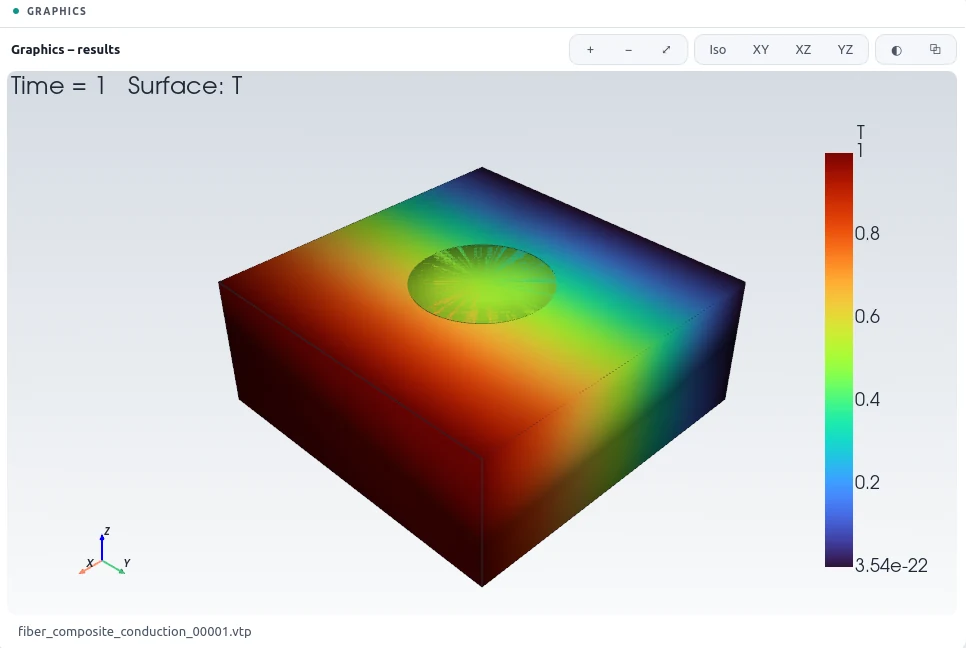
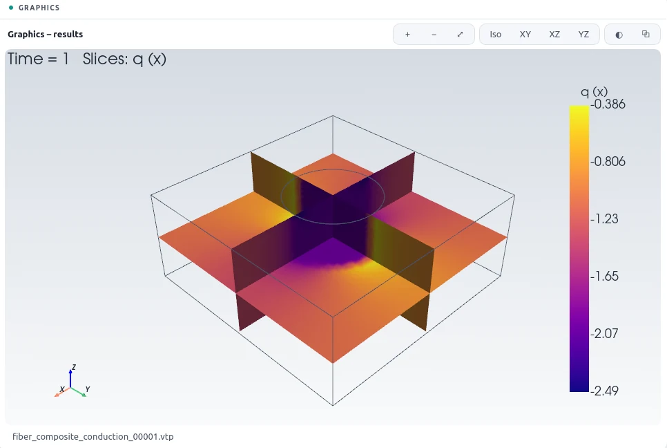
A square array of fibres, ten times more conductive than the matrix, occupies 12.6 % of the volume. Its unit cell is a box with one fibre through the middle; by symmetry, a temperature difference across the cell and insulated sides give the response of the whole array, and the mean heat flux gives its effective conductivity. Rayleigh's classical solution for a square array is 1.2292 times the matrix conductivity.
2The Problem File
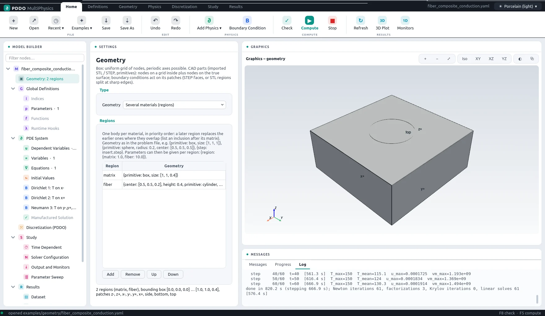
Instead of one geometry, the domain lists regions: the matrix box and then the
fibre cylinder. A later region replaces an earlier one where they overlap, and their common surface
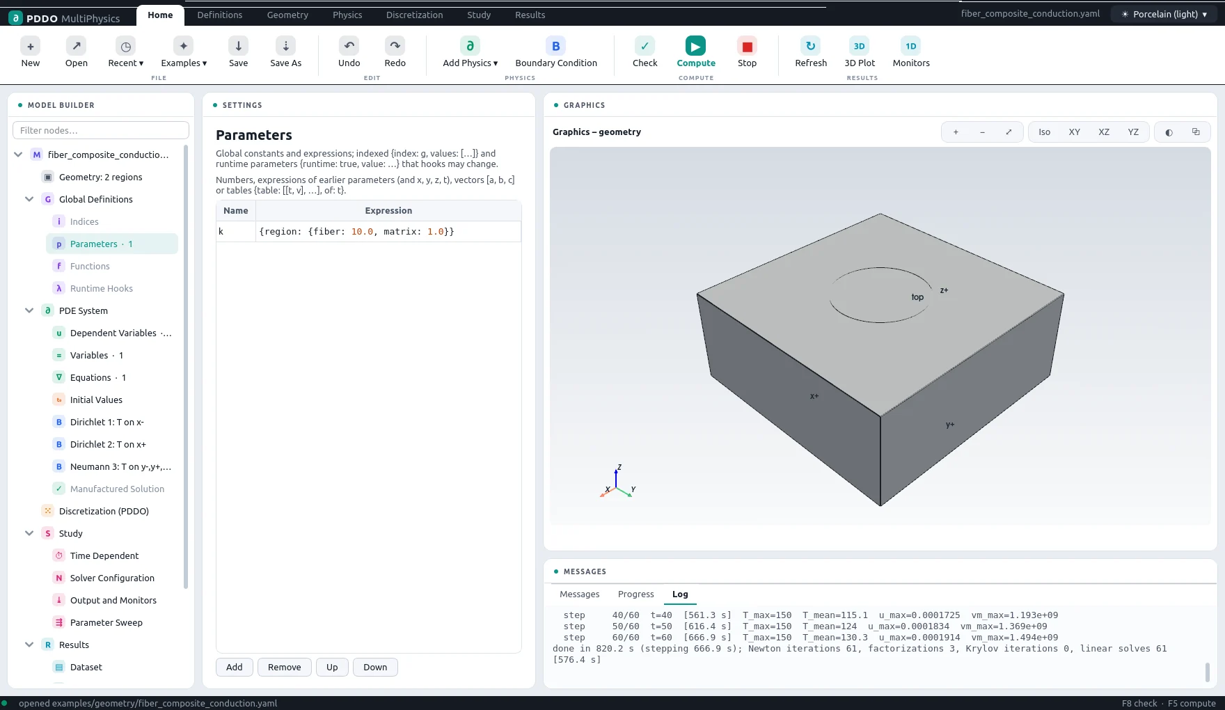
becomes an interface. A parameter can take a value per region, k: {region: {matrix: 1.0,
fiber: 10.0}}. The interface conditions need no input: the engine reads the flux from the
div() term of the equation and makes it continuous across the interface, along with the
temperature.
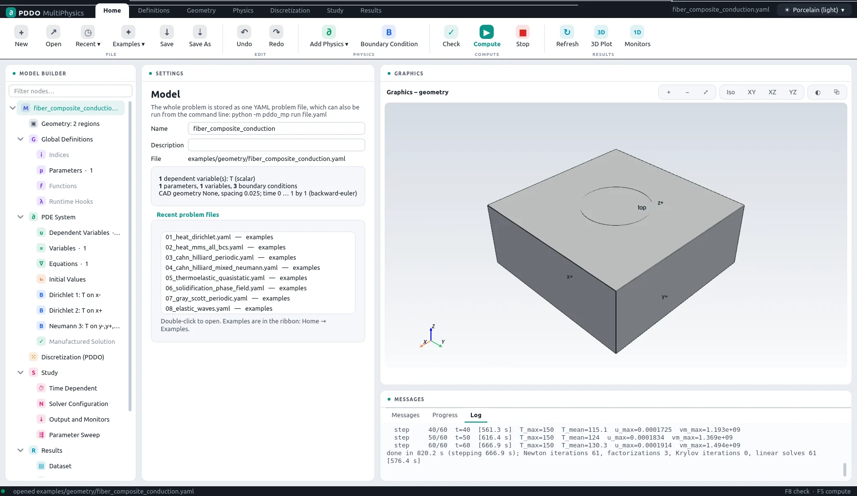
The complete problem file, examples/geometry/fiber_composite_conduction.yaml
# Two materials (regions): transverse heat conduction through a unit cell of a fiber
# composite (square array of fibers, fiber volume fraction f = pi r^2 = 0.126).
#   div(k grad T) = 0,   k = 1 (matrix), 10 (fiber)
# The cell boundaries are symmetry planes of the array: T = 0 / 1 on x- / x+, insulated
# elsewhere. The effective conductivity is the mean flux (monitor k_eff); Rayleigh's
# formula for a square array: k_eff = 1 + 2f / (1/b - f - 0.3058 b f^4),
# b = (k_f - k_m)/(k_f + k_m)  ->  1.2292.
# The fiber is listed after the matrix: it replaces the matrix where they overlap. Its
# surface becomes the interface (continuity of T and of k grad(T).n); its end faces lie on
# the cell faces z- / z+ and keep the names bottom / top.
"k">name: fiber_composite_conduction
"k">domain:
  "k">type: geometry
  "k">spacing: 0.025                # fiber radius = 8 spacings; 0.035 -> +1.6 %, 0.025 -> +0.5 %
  "k">regions:
    - "k">name: matrix
      "k">geometry: {primitive: box, size: [1, 1, 0.4]}
    - "k">name: fiber
      "k">geometry: {primitive: cylinder, radius: 0.2, height: 0.4, center: [0.5, 0.5, 0.2]}
"k">parameters:
  "k">k: {region: {matrix: 1.0, fiber: 10.0}}
"k">fields:
  "k">T: scalar
"k">relations:
  "k">q: "-k*grad(T)"                 # heat flux
"k">equations:
  "k">T: "div(k*grad(T)) = 0"
"k">boundary_conditions:
  - "k">faces: [x-]
    "k">T: {dirichlet: 0}
  - "k">faces: [x+]
    "k">T: {dirichlet: 1}
  - "k">faces: [y-, y+, z-, z+, bottom, top]
    "k">T: {neumann: 0}
"k">time:
  "k">end: 1
  "k">dt: 1
  "k">scheme: backward-euler
"k">output:
  "k">fields: [T, q]
"k">monitors:
  "k">k_eff: "mean(k*dx(T))"
3Discretization
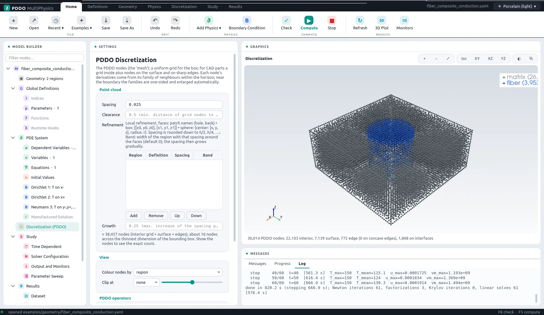
With a spacing of 0.025 the cell holds 30,014 nodes. Nodes on the interface come in pairs, one for each material, with opposite normals; the families of each region stay inside it.
4Results
- Nodes
- 30,014 (point cloud)
- PDDO order
- 2, horizon 2.015 Δx
- Time scheme
- backward-euler
- Steps
- 1 × Δt = 1
- Newton iterations
- 1
- Factorizations
- 1
- Run time
- 61 s
The computed effective conductivity is 1.2350, +0.47 % from Rayleigh's value. With a coarser spacing of 0.035 the difference is +1.6 %: it falls with refinement, as it should.
5Run It Yourself
The problem file ships with PDDO-MultiPhysics. Open it in the graphical interface and press Compute, or run it from the command line:
python -m pddo_mp gui examples/geometry/fiber_composite_conduction.yaml
python -m pddo_mp run examples/geometry/fiber_composite_conduction.yaml
Results go to results/fiber_composite_conduction/
next to the problem file: a ParaView time series (.pvd), the monitors as CSV, and the
final state. Any entry can be changed on the command line, for example
--set domain.spacing=0.05 for a coarser, faster run. The user manual
describes every part of the problem file and of the interface.