Viscoelastic creep of a bar | PDDO-MultiPhysics Examples

1The Problem

A bar of a viscoelastic material is suddenly loaded with a constant stress and held. It responds at once with the stiffness of both springs, then creeps towards the strain of the long-term spring alone, with a retardation time that the model predicts exactly.

$$\boldsymbol{\sigma} = \mathbb{C}_0 : \boldsymbol{\varepsilon} + \mathbb{C}_1 : (\boldsymbol{\varepsilon} - \boldsymbol{\varepsilon}^v), \qquad \frac{\partial \boldsymbol{\varepsilon}^v}{\partial t} = \frac{\boldsymbol{\varepsilon} - \boldsymbol{\varepsilon}^v}{\tau}$$

$$\varepsilon(t) = \frac{s_0}{E_0} - s_0\Big(\frac{1}{E_0} - \frac{1}{E_0 + E_1}\Big)\,e^{-t/\tau_r}, \qquad \tau_r = \tau\,\frac{E_0 + E_1}{E_0}$$

2The Problem File

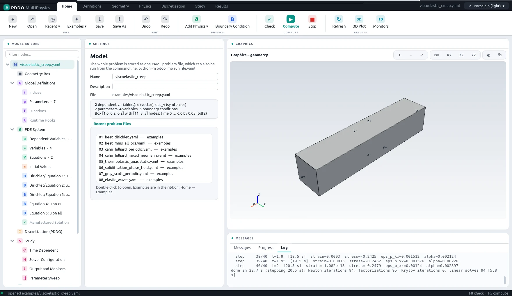
The viscous strain is a symmetric-tensor field, eps_v: symtensor, with its own evolution equation and no spatial derivative: a local ODE at every node, solved together with equilibrium. The bar's three symmetry planes fix one displacement component each, written as a component condition such as u_x: {dirichlet: 0} alongside zero traction.

The complete problem file, examples/viscoelastic_creep.yaml

# Viscoelasticity (standard linear solid / Zener, 3D, internal variable as a local ODE):
#   sigma = C0 : eps + C1 : (eps - eps_v),     dt(eps_v) = (eps - eps_v)/tau,   C1 = beta C0
# Creep of a bar under a constant end stress s0 (symmetry planes x-, y-, z-):
#   eps(t) = s0/E0 - s0 (1/E0 - 1/(E0 + E1)) exp(-t/tau_r),  tau_r = tau (E0 + E1)/E0
"k">name: viscoelastic_creep
"k">domain:
  "k">size: [1.0, 0.2, 0.2]
  "k">n: [11, 5, 5]
"k">parameters:
  "k">E0: 100.0
  "k">beta: 2.0                        # E1 = beta E0
  "k">nu: 0.3
  "k">tau: 1.0
  "k">s0: 0.1
  "k">lambda: "E0*nu/((1 + nu)*(1 - 2*nu))"
  "k">G: "E0/(2*(1 + nu))"
"k">fields:
  "k">u: vector
  "k">eps_v: symtensor
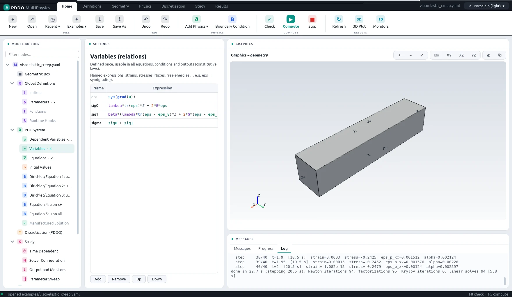
"k">relations:
  "k">eps: "sym(grad(u))"
  "k">sig0: "lambda*tr(eps)*I + 2*G*eps"
  "k">sig1: "beta*(lambda*tr(eps - eps_v)*I + 2*G*(eps - eps_v))"
  "k">sigma: "sig0 + sig1"
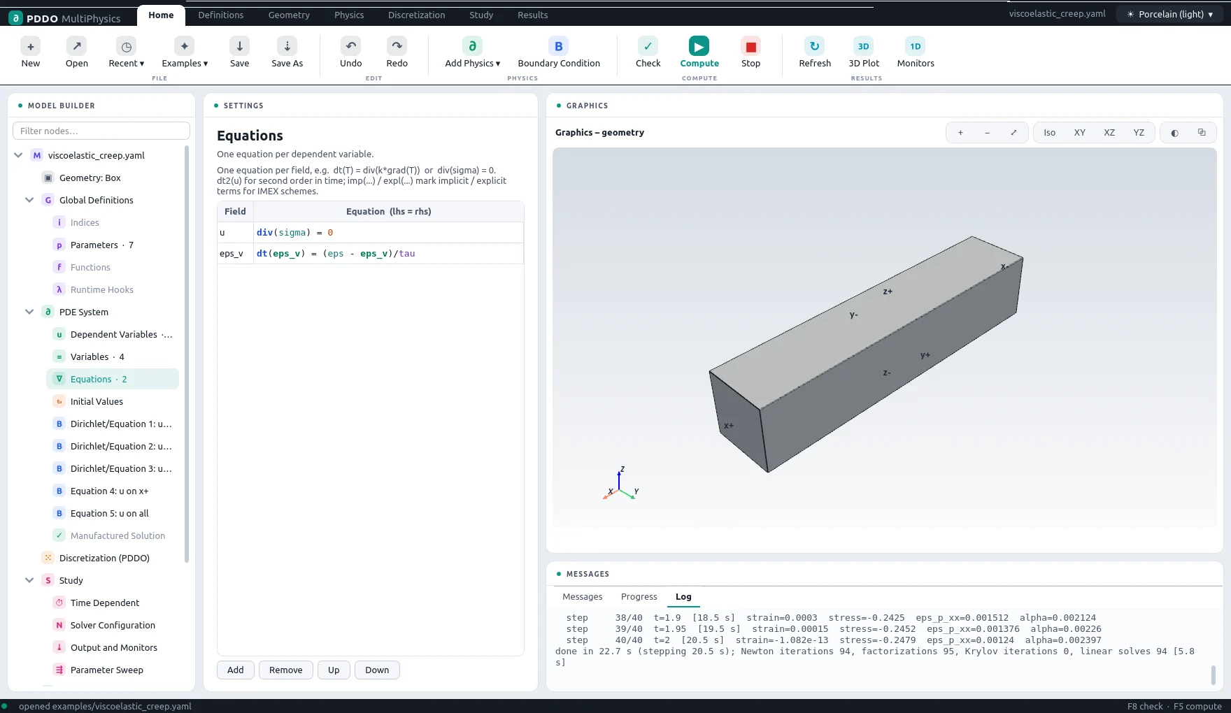
"k">equations:
  "k">u: "div(sigma) = 0"
  "k">eps_v: "dt(eps_v) = (eps - eps_v)/tau"
"k">boundary_conditions:
  - "k">faces: [x-]
    "k">u: {equation: "dot(sigma, n) = [0, 0, 0]"}
    "k">u_x: {dirichlet: 0}
  - "k">faces: [y-]
    "k">u: {equation: "dot(sigma, n) = [0, 0, 0]"}
    "k">u_y: {dirichlet: 0}
  - "k">faces: [z-]
    "k">u: {equation: "dot(sigma, n) = [0, 0, 0]"}
    "k">u_z: {dirichlet: 0}
  - "k">faces: [x+]
    "k">u: {equation: "dot(sigma, n) = [s0, 0, 0]"}
  - "k">faces: all
    "k">u: {equation: "dot(sigma, n) = [0, 0, 0]"}
"k">time:
  "k">end: 6.0
  "k">dt: 0.05
  "k">scheme: bdf2
"k">output:
  "k">every: 20
"k">monitors:
  "k">strain: "mean(eps[0, 0])"
  "k">stress: "mean(sigma[0, 0])"

**Figure 1.** The model in the GUI: the Model Builder tree on the left, the settings of the selected node in the middle, the graphics window on the right.

**Figure 2.** Elastic and viscous stress contributions.

**Figure 3.** Equilibrium and the evolution of the viscous strain.

3Results

Nodes: 11×5×5 = 275
PDDO order: 2, horizon 2.015 Δx
Time scheme: bdf2
Steps: 120 × Δt = 0.05
Newton iterations: 121
Factorizations: 3
Run time: 4 s

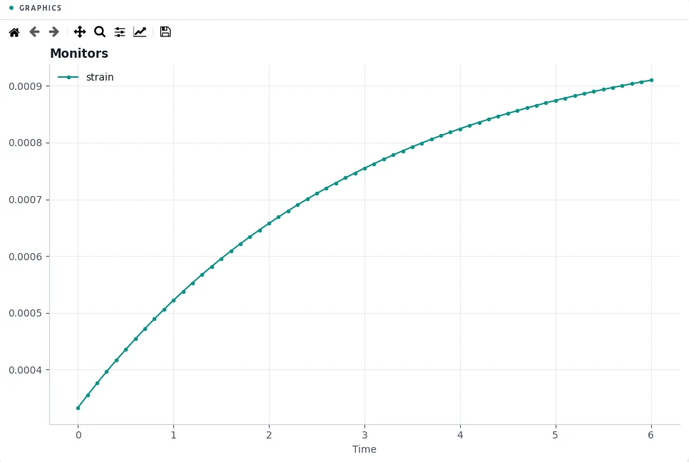
This run stored every output step for the plots: --set output.every=2 on the command line; the problem file itself writes less often.

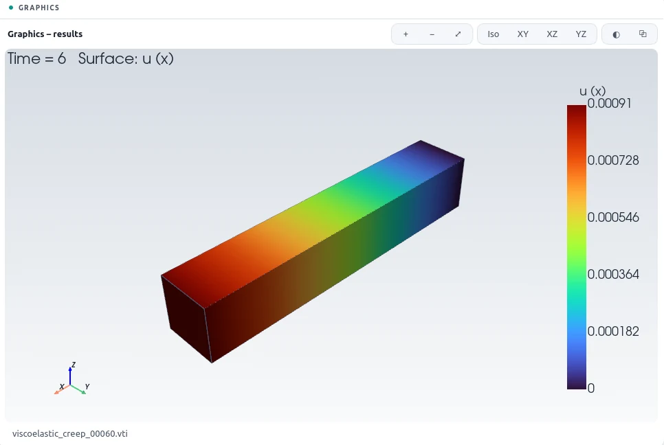
The strain jumps to 3.333×10^-4 on loading and creeps to 9.098×10^-4 at the end of the run, approaching the long-term value 0.001000 with the retardation time τ_r = 3.0. The largest difference from the analytic curve is 0.013 % of the long-term strain.

**Figure 4.** Mean axial strain against time: the creep curve.

**Figure 5.** Axial displacement on the deformed bar at the final time.

4Run It Yourself

The problem file ships with PDDO-MultiPhysics. Open it in the graphical interface and press Compute, or run it from the command line:

python -m pddo_mp gui examples/viscoelastic_creep.yaml
python -m pddo_mp run examples/viscoelastic_creep.yaml --set output.every=2

Results go to results/viscoelastic_creep/ next to the problem file: a ParaView time series (.pvd), the monitors as CSV, and the final state. Any entry can be changed on the command line, for example --set time.end=3 for a run to half the end time. The user manual describes every part of the problem file and of the interface.

1The Problem

2The Problem File

3Results

4Run It Yourself

Have a coupled problem of your own?