Thermoelastic block heated on one face | PDDO-MultiPhysics Examples

1The Problem

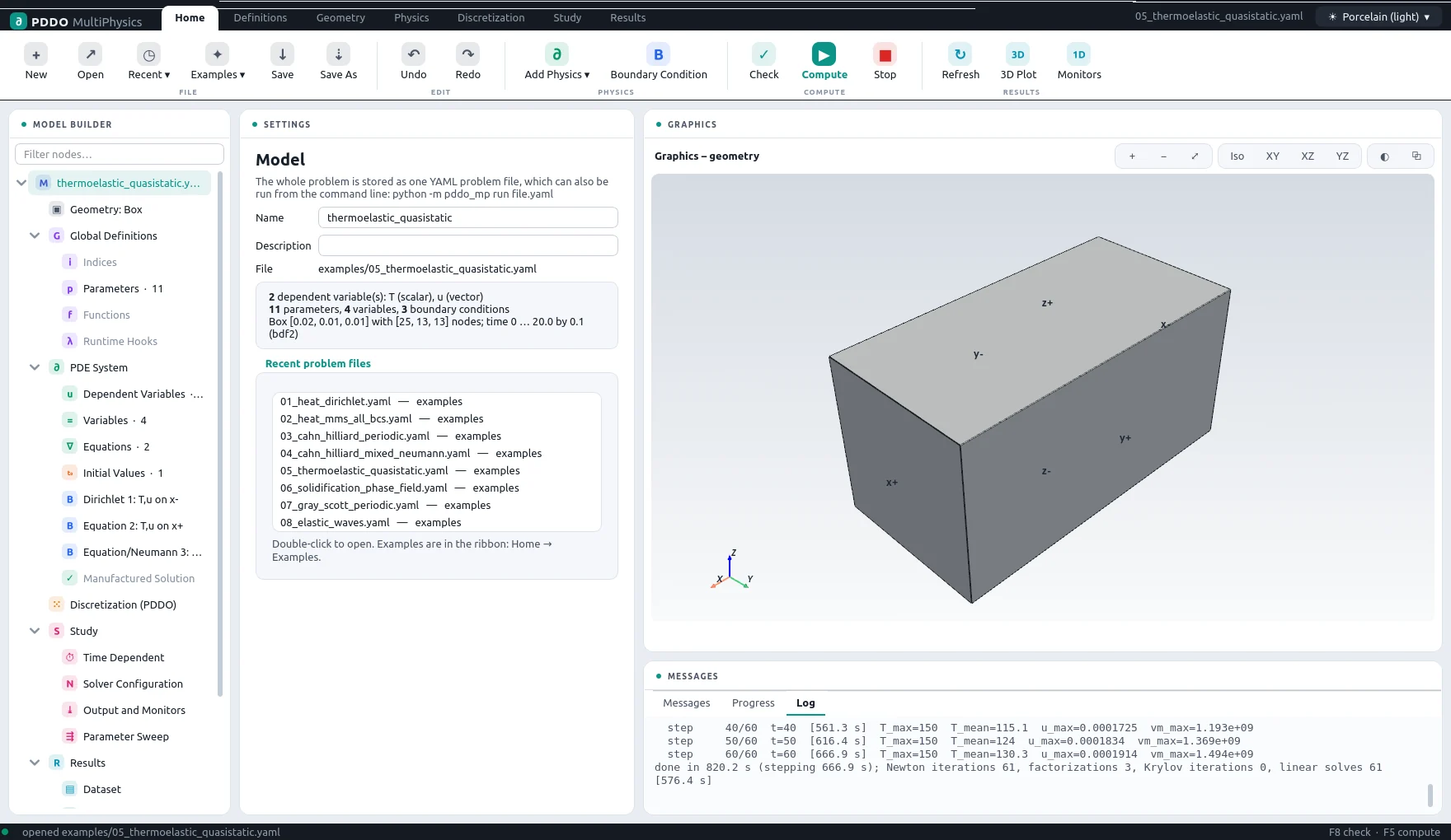
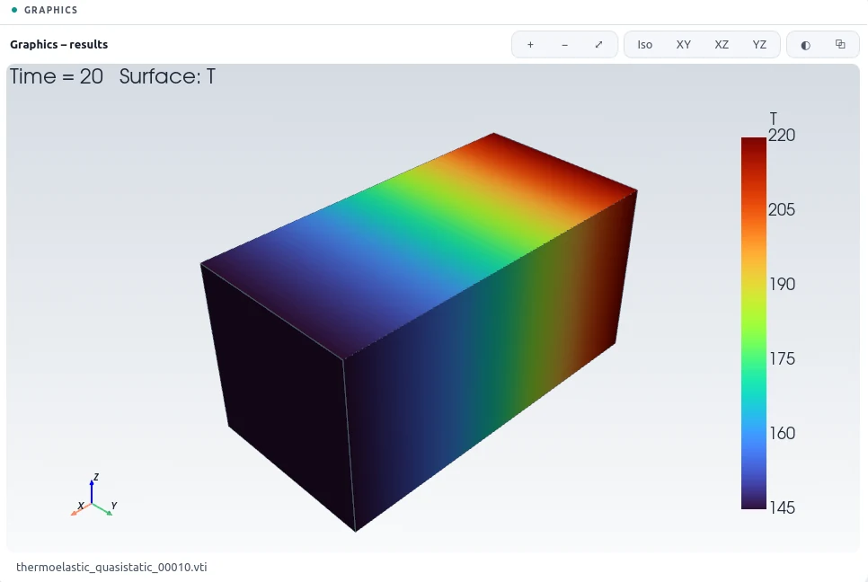
A 20×10×10 mm steel block is clamped at x−, where its temperature is ramped from 20 to 220 °C over two seconds. The opposite face loses heat to the surroundings by convection; the side faces are insulated and, mechanically, every face except the clamped one is free. As the heat spreads, the block expands and the constraint of the clamped face produces thermal stress.

$$\rho c_p\,\frac{\partial T}{\partial t} = -\nabla\cdot\mathbf{q}, \qquad \mathbf{q} = -k\,\nabla T$$

$$\nabla\cdot\boldsymbol{\sigma} = \mathbf{0}, \qquad \boldsymbol{\sigma} = \lambda\,\mathrm{tr}(\boldsymbol{\varepsilon})\,\mathbf{I} + 2G\,\boldsymbol{\varepsilon} - (3\lambda + 2G)\,\alpha\,(T - T_0)\,\mathbf{I}, \qquad \boldsymbol{\varepsilon} = \tfrac12(\nabla\mathbf{u} + \nabla\mathbf{u}^{\mathsf T})$$

2The Problem File

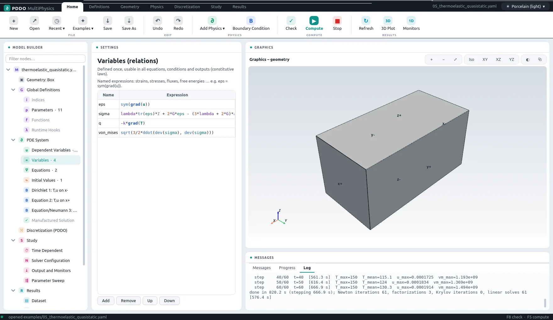
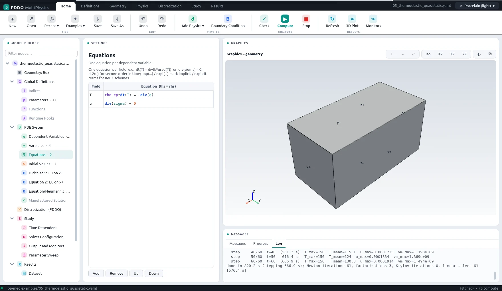
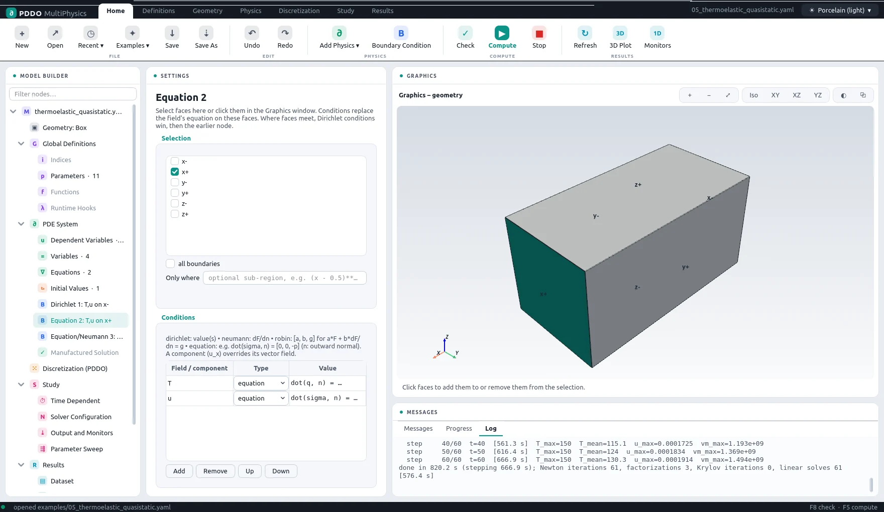
Two fields, T: scalar and u: vector, and four relations: the strain sym(grad(u)), the stress, the heat flux and the von Mises stress. The traction-free faces are written as equations in the stress and the outward normal, dot(sigma, n) = [0, 0, 0], and the convective face as dot(q, n) = h_conv*(T - T0). The Lamé constants are derived parameters, expressions in E and nu.

Everything is linear with constant coefficients, so with the implicit BDF2 scheme the system matrix is assembled once and factorized only 3 times in the whole run (the start-up steps of BDF2 use different coefficients); every other step reuses a factorization.

The complete problem file, examples/05_thermoelastic_quasistatic.yaml

# Thermo-mechanics: transient heat conduction + quasi-static linear thermoelasticity.
#   rho*cp*dt(T) = div(k grad T)
#   div(sigma) = 0,  sigma = lambda tr(eps) I + 2 G eps - (3 lambda + 2 G) alpha (T - T0) I
#   eps = sym(grad u)                      (small strain)
# A block is heated on face x- (temperature ramped to T_hot) and cools by convection on
# x+; the other faces are insulated. Mechanically, x- is clamped, all other faces are
# traction free. Units: SI with mm-scale block (values are illustrative).
#
# Everything is linear with constant coefficients, so with an implicit scheme the system
# matrix is built and factorized once and reused for every step.
"k">name: thermoelastic_quasistatic
"k">domain:
  "k">size: [0.02, 0.01, 0.01]
  "k">n: [25, 13, 13]
"k">parameters:
  "k">E: 200.0e9
  "k">nu: 0.3
  "k">alpha: 12.0e-6
  "k">k: 45.0
  "k">rho_cp: 3.6e6
  "k">h_conv: 500.0
  "k">T0: 20.0
  "k">T_hot: 220.0
  "k">t_ramp: 2.0
  "k">lambda: "E*nu/((1 + nu)*(1 - 2*nu))"
  "k">G: "E/(2*(1 + nu))"
"k">fields:
  "k">T: scalar
  "k">u: vector
"k">relations:
  "k">eps: "sym(grad(u))"
  "k">sigma: "lambda*tr(eps)*I + 2*G*eps - (3*lambda + 2*G)*alpha*(T - T0)*I"
  "k">q: "-k*grad(T)"
  "k">von_mises: "sqrt(3/2*ddot(dev(sigma), dev(sigma)))"
"k">equations:
  "k">T: "rho_cp*dt(T) = -div(q)"
  "k">u: "div(sigma) = 0"
"k">boundary_conditions:
  - "k">faces: [x-]
    "k">T: {dirichlet: "T0 + (T_hot - T0)*min(t/t_ramp, 1)"}
    "k">u: {dirichlet: [0, 0, 0]}
  - "k">faces: [x+]
    "k">T: {equation: "dot(q, n) = h_conv*(T - T0)"}
    "k">u: {equation: "dot(sigma, n) = [0, 0, 0]"}
  - "k">faces: [y-, y+, z-, z+]
    "k">T: {neumann: 0}
    "k">u: {equation: "dot(sigma, n) = [0, 0, 0]"}
"k">initial_conditions:
  "k">T: "T0"
"k">time:
  "k">end: 20.0
  "k">dt: 0.1
  "k">scheme: bdf2
"k">output:
  "k">every: 20
  "k">fields: [T, u, sigma, von_mises]
"k">monitors:
  "k">T_mean: "mean(T)"
  "k">ux_tip_max: "max(u_x)"
  "k">vm_max: "max(von_mises)"

**Figure 1.** The model in the GUI: the Model Builder tree on the left, the settings of the selected node in the middle, the graphics window on the right.

**Figure 2.** Variables: strain, thermoelastic stress, heat flux and von Mises stress.

**Figure 3.** The two equations: transient heat conduction and quasi-static equilibrium.

**Figure 4.** The x+ face: convection for T and zero traction for u, both written as equations in the outward normal n.

3Results

Nodes: 25×13×13 = 4,225
PDDO order: 2, horizon 2.015 Δx
Time scheme: bdf2
Steps: 200 × Δt = 0.1
Newton iterations: 201
Factorizations: 3
Run time: 63 s

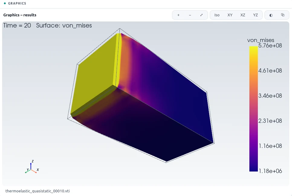
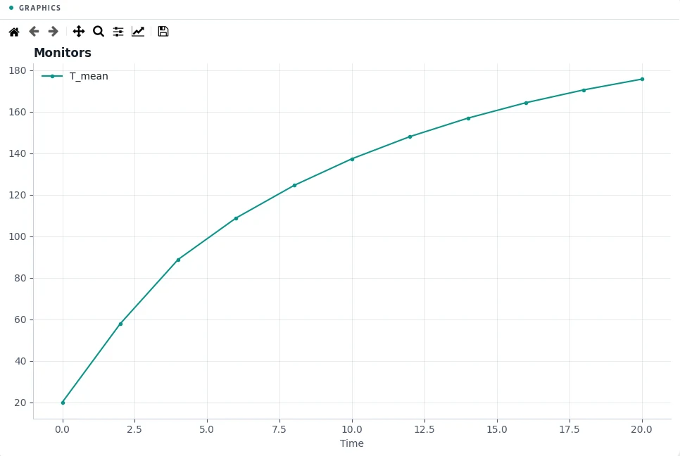
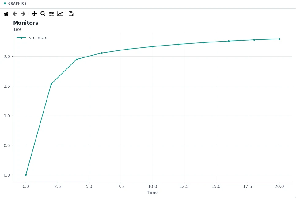
After 20 seconds the mean temperature of the block has risen to 176 °C and the free end has moved by 40.6 µm along x. The thermal stress is largest where the expansion is fully constrained, at the clamped face: 99 % of the block is below 1464 MPa von Mises. The single largest value, 2297 MPa, sits on the edges of the clamped face, where a clamped linear-elastic model has a stress singularity and the peak grows with refinement.

**Figure 5.** Temperature at t = 20 s: hot at the clamped face, cooled by convection at the free end.

**Figure 6.** Von Mises stress on the deformed block, seen from the clamped face (colour range limited to the 95th percentile; the peak sits at the clamped edges).

**Figure 7.** Mean temperature against time.

**Figure 8.** Largest von Mises stress against time.

4Run It Yourself

The problem file ships with PDDO-MultiPhysics. Open it in the graphical interface and press Compute, or run it from the command line:

python -m pddo_mp gui examples/05_thermoelastic_quasistatic.yaml
python -m pddo_mp run examples/05_thermoelastic_quasistatic.yaml

Results go to results/thermoelastic_quasistatic/ next to the problem file: a ParaView time series (.pvd), the monitors as CSV, and the final state. Any entry can be changed on the command line, for example --set time.end=10 for a run to half the end time. The user manual describes every part of the problem file and of the interface.

1The Problem

2The Problem File

3Results

4Run It Yourself

Have a coupled problem of your own?